Atmospheric and Climate Sciences
Vol.3 No.1(2013), Article ID:27580,11 pages DOI:10.4236/acs.2013.31012
Characterizing PM2.5 Pollution of a Subtropical Metropolitan Area in China
1Department of Chemical and Biological Engineering, Zhejiang University, Hangzhou, China
2Environmental Monitoring Center, Hangzhou, China
3Zhejiang Environmental Protection Agency, Hangzhou, China
Email: *yihezj@zju.edu.cn
Received November 30, 2012; revised December 27, 2012; accepted January 5, 2013
Keywords: PM Pollution; PM2.5 Composition; Breathing Zone; Air Pollution Measurements; Personal Exposure
ABSTRACT
The chemical and physical characteristics of PM2.5, especially their temporal and geographical variations, have been explored in metropolitan Hangzhou area (China) by a field campaign from September 2010 to July 2011. Annual average concentrations of PM2.5 and PM10 during non-raining days were 106 - 131 µg∙m−3 and 127 - 158 µg∙m−3, respectively, at three stations in urban breathing zones, while corresponding concentrations of PM2.5 and PM10 at an urban background station (16 m above ground level in a park) were 78 and 104 µg∙m−3, respectively. For comparison, the annual average PM10 concentration at a suburban station (5 m AGL) was 93 µg∙m−3. Detailed chemical analyses were also conducted for all samples collected during the campaign. We found that toxic metals (Cd, As, Pb, Zn, Mo, Cu, Hg) were highly enriched in the breathing zones due to anthropogenic activities, while soluble ions ( ,
,  ,
, ) and total carbon accounted for majority of PM2.5 mass. Unlike most areas in China where sulfate was several times of nitrate in fine PM, nitrate was as important as sulfate and highly correlated with ammonium during the campaign. Thus, a historical shift from sulfate-dominant fine PM to nitrate-dominant fine PM was documented.
1. Introduction
PM2.5 is an important air pollutant. Due to its relatively long suspension time in the air and special optical properties, PM2.5 is responsible for the formation of regional haze [1-3]. Depending on its position in the air, PM2.5 may be responsible for warming or cooling of surface [4]. When inhaled, PM2.5 may cause severe health problems, such as asthma, lung cancer, and heart disease [5-10], though the exact component of PM2.5 responsible for certain adverse health effect is uncertain [8,9].
To protect the public from PM2.5 pollution, significant efforts have been conducted worldwide [11-15]. For example, US EPA has started to regulate ambient PM2.5 pollution since 1998, and recently tightened its ambient air quality standards for 24-hour and annual averages to 35 and 15 µg∙m−3 [16], respectively. As PM2.5 pollution started to draw public attention in China, China Ministry of Environmental Protection recently released its first ambient air quality standard for PM2.5, to be effective in 2016; the standard sets the same PM2.5 limits for recreational areas as US EPA, but allows non-recreational areas to have higher limits, namely, 70 and 35 µg∙m−3 for 24-h and annual averages, respectively.
While intensive field campaigns have been carried out in China and elsewhere [17-20], the temporal and geographical variations of PM2.5 in urban breathing zones (0.5 - 2 m above ground) in China remain poorly documented. To obtain such detailed information about PM2.5 pollution, an extensive field campaign was conducted in metropolitan Hangzhou area (HZ), China, during September 2010-July 2011. HZ is experiencing both fast urbanization and growing environmental issues: as of 2010, the population of HZ ranked sixth in China, and the population density was 1214/km2. The goals of this campaign were: 1) to determine the pollution level of PM2.5 in the breathing zone of urban air; 2) to investigate chemical and physical characteristics of PM2.5 pollution; 3) to identify areas for further research before next field campaign. Section 2 will describe experimental methods of the campaign, and Section 3 will present major findings. A summary will be presented in Section 4.
2. Experimental Methods
The sampling, analysis, and quality assurance procedures are described below.
2.1. Sampling
2.1.1. Sites
HZ is situated in a subtropical area with distinct seasonal weather conditions, and is 50-km away from the western rim of the Pacific Ocean. As HZ is a traditional hotspot for national and international tourists, there are two automatic monitoring stations (“A” and “B”, Table 1) running since 2005 for PM2.5 as well as other air pollutants, independent of this campaign: one (“A”) represents suburban recreational conditions, and the other (“B”) represents urban mixed conditions. Sampling inlets were at 5 m (“A”) and 16 m (“B”) above ground level (AGL) at the automatic stations. For this campaign, four additional stations were chosen to represent breathing zone conditions in various urban areas, namely, nearby highway (“C”), a college gate (“D”), a business area with peak hours (“E”), and a business area without peak hours but with dense population (“F”). At these special stations, sampling inlets were at 1 - 1.5 m AGL. Figure 1 shows the sampling sites for this campaign.
2.1.2. Duration
Sampling was conducted at all stations from September 2010 to July 2011. During the sampling period, seasonal average temperatures in the area were 21˚C for fall (September-November 2010), 6.9˚C for winter (December 2010-February 2011), 16˚C for spring (March-May 2011), and 29˚C for summer (June-August 2011). As it was raining frequently in the sampling region, PM2.5 samples were only collected at sites “A”-“E” concurrently during non-raining days. On each sampling day, samples were collected for 18 - 24 hours; in each season, 7 - 10 days were selected for concurrent sampling. In addition, PM2.5 samples were also collected at sites “B” and “F” during January-June 2008.
2.1.3. Samplers
At sites “A”, “B”, “F”, air pollutants were continuously measured for PM2.5, O3, CO, NO2, CH4, and NMHC, using automatic monitoring equipment (Air Point, Austria; DURAG, Germany; SYNSPEC, Holland). At sites specially selected for this campaign, PM2.5 samplers were the model TH-150C, manufactured by Wuhan Tianhong Instruments Co., Ltd. The operational volume flow rate for PM2.5 samplers was set at 100 L∙min−1, and the size cut was at 2.5 µm. At each site, three samplers were used to collect three concurrent PM2.5 samples for analyzing inorganic elements, soluble ions, and carbon items, respectively. For inorganic elemental analysis, PTEF organic filters (Sumitomo Electric Fine Polymer, Inc.) were used. For organic analyses, quartz filters (Whatman 1851047) were used. The pore size was 0.3 µm for both types of filters, and the collection efficiency at 0.15 µm was 99.97% for organic filters and 99% for quartz filters.
2.2. Analyses
The bulk masses of PM2.5 samples were weighed with a balance (0.0001 accuracy), and the speciation was conducted for 25 inorganic elements, 9 ions, and 3 carbon items. Details are elaborated below.
Table 1. PM concentration in a subtropical metropolitan area (HZ, CHINA).
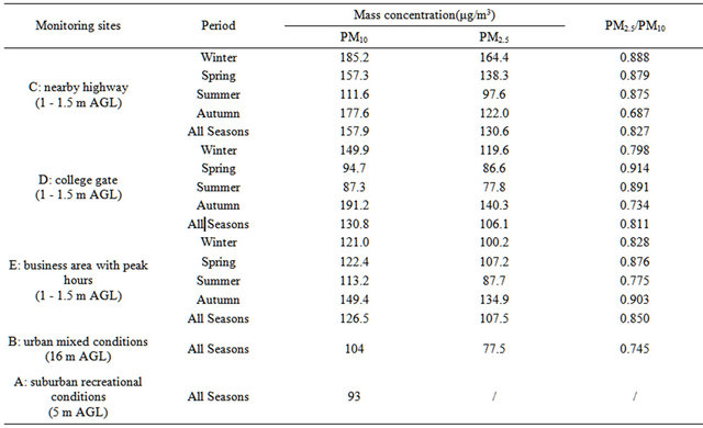
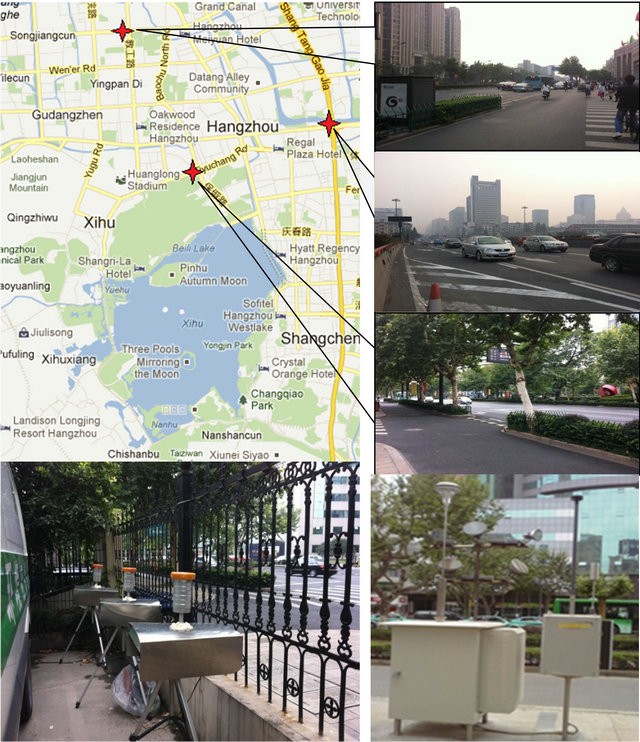
Figure 1. Monitoring stations and sampling setup. The distributions of the sampling locations are marked with red stars in the Google map.
2.2.1. Inorganic Elements
After sampling, organic filters loaded with PM2.5 were carefully cut along the inner rim and put into a 50 ml microwave digestion tank. 6 ml HNO3 and 2 ml H2O2 were then added into the tank to dissolve PM2.5 at predesigned procedures. Then, the bulk solution was moved into a 50 mL flask. High-purity water was used to fix the volume and for mixing well. Finally, the solution was used for instrumental analyses.
Instrumental analyses were conducted by Inductively Coupled Plasma (ICP, Optima 7300DV) emission spectrometers for elements (Li, V, Cr, Co, Ni, Cd), by Atomic Fluorescent Spectrometers (AFS-9230) for elements (Hg, As, Se), and by ICP-Mass Spectrometers (MS, X Series 2) for elements (Al, Ba, Ca, Cu, Fe, K, Mg, Mn, Mo, Na, P, Pb, S, Si, Ti, Zn).
For the AFS analysis, sample solutions were first heated in acidic media to convert all mercury into Hg2+, and Hg2+ was then reduced by KBH4 to form Hg vapor that was drawn into AFS for detection. As and Se were detected similarly.
2.2.2. Soluble Ions
After sampling, a piece of organic filters loaded with PM2.5 were put into a 25-ml colorimetric tube. Then, 20.00-ml deionized water was added to and bubbles expelled from the tube. The tube was placed in a supersonic cleaner running for 20 minutes. After stilled for a while, clear solution in top layer was drawn and filtered before being analyzed by Ion Chromatography for water-soluble anions (F−, Cl−,  ,
, ; Dionex IC DX600) and cations (NH4+, K+, Na+, Ca2+, Mg2+; Dionex ICS-90).
2.2.3. Carbon Analysis
After sampling, quartz filters loaded with PM2.5 were put on new and clean aluminum foil, and a representative piece was obtained carefully. A second piece with the same area was obtained and processed as follows to remove carbonate. First, the second piece was merged in concentrated HCl solution in a covered container. Then, the container was placed in a ventilator cabinet for about an hour to remove carbonate in the form of CO2 and for another hour to let remaining HCl evaporate. The sample was then kept at low temperature and saved for subsequent analyses.
The organic, elemental, and total carbon contents of PM2.5 samples were determined with a thermo-photometric carbon analyzer (DRI Model 2001A). A piece of processed sample filter (0.495 cm2) was put in an environment with pure He gas without O2, and was heated progressively at 120˚C, 250˚C, 450˚C, and 550˚C first to determine organic carbon contents OC1, OC2, OC3, and OC4, respectively. Then, in an environment with 2% O2 and 98% He, the sample was further heated progressively at 550˚C, 700˚C, and 800˚C to determine elemental carbon contents EC1, EC2, and EC3. The CO2 produced within each temperature ladder was reduced into CH4, catalyzed by MnO2, for being detected with Fire Ionization Detectors. During heating processes, part of organic carbon was converted into black carbon, which hindered clear distinction between organic carbon and elemental carbon. Hence, the reflection intensity of the He-Ne laser light at 633 nm by a monitoring filter was used to gauge the starting temperature of the oxidation of elemental carbon, to ensure science-based distinction between organic carbon and elemental carbon.
2.3. QA/QC Procedures
2.3.1. Sampling
All sampling instruments used for this study were calibrated by the Technology Supervision Bureau of Zhejiang Province within valid periods. Before each sampling, pump volumes of PM2.5 samplers were calibrated, and so were sampling volumes of other instruments. During filter sampling, a specialist was responsible for checking conditions of volume-flow meters of sampling pumps, and the project manager randomly checked conditions of flow meters at a frequency. Records were made to ensure the precision of sampling volumes and subsequent calculations of pollutant concentrations. No sample was collected in raining weather, and filter samples were ensured to conserve particulate matter during transportation.
2.3.2. Weighing
Before and after sampling, organic filters were baked at 60˚C ± 2˚C for 8 hours and blank quartz filters were baked at 500˚C for 4 hours. Then, filters were put in dryers for at least 48 hours before weighing. This procedure is expected to remove the disturbance of water, and to provide weighting results comparable with other studies though some compounds such as ammonium nitrate may evaporate if original samples were collected at relatively humid condition, e.g., when relative humidity was over 80%. During weighing, samples were put into glass agar plates and covered to avoid the effect of static electricity.
2.3.3. Elemental Analyses
Each container used for this study was cleaned first, and then washed with warm, 10% HNO3. Then, the container was rinsed with tap water. Finally, the container was rinsed repeatedly with deionized water (Mill-Q, >18.2 MΩ·cm at 25˚C), in order to reduce blank background. For each batch of samples, at least three blank samples were analyzed to determine blank background value. During sample analyses, a standard sample was added for every 10 - 15 samples, to check instrumental stability. When an element showed abnormally high content, analysis was stopped and the inlet system was rinsed with 2% HNO3 Then, standard solutions were used to calibrate instruments, and samples were diluted before subsequent analyses.
2.3.4. Ionic Analyses
Glass containers were cleaned, and soaked in deionized water for over 24 hours. Then, containers were cleaned with supersonic waves for 30 minutes. Blank background was determined in the same way as for elemental analyses, and so was the use of standard samples.
2.3.5. Carbon Analysis
At the beginning and the end of each day when samples were analyzed, CH4/CO2 standard gases were used to calibrate instruments. For every 10 samples, one was randomly chosen for parallel analysis. Two standard samples were analyzed every two weeks. Compared with DRI (USA) instruments which have the same model or use different methods [21-28], the detection precision was <5% for TC and <10% for OC and EC in this study.
3. Results and Discussions
PM mass concentrations and PM2.5 compositions are presented below.
3.1. Mass Concentration
Table 1 lists average PM concentrations in the metropolitan breathing zones, at an urban background station, and at a suburban background station during this campaign. It is shown that the average PM2.5 concentration in the breathing zone ranged from 106 to 131 µg∙m−3 annually and from 78 to 164 µg∙m−3 seasonally, with peak values nearby highway in winter and in business areas in fall. PM2.5 accounted for 81% - 85% of PM10 annually and 69% - 91% of PM10 seasonally. Concentrations of PM2.5 and PM10 at the metropolitan background station (16 m AGL in a park) were lower than in the breathing zones by (27 - 41)% and (18 - 34)%, respectively. The concentration of PM with diameters between 2.5 - 10 µm was ~25 µg∙m−3 in urban stations during the campaign.
3.2. Elemental Composition
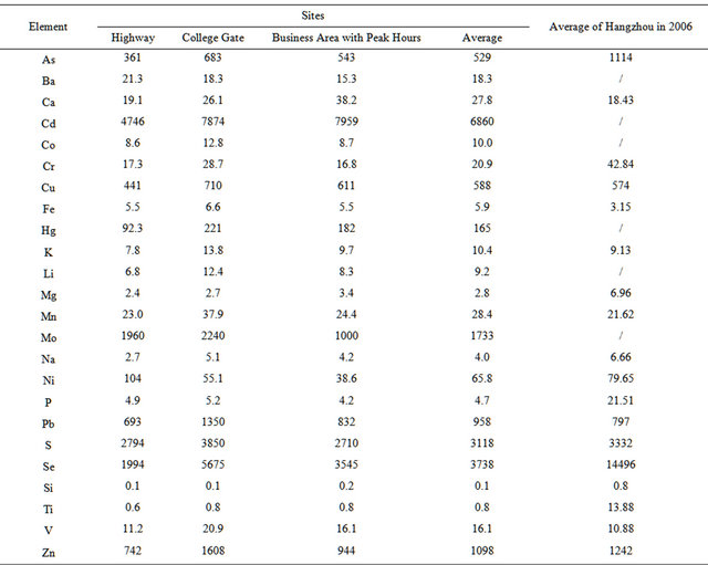
Table 2 lists concentrations of 25 elements detected in PM2.5 samples collected in the breathing zones during the campaign. A number of metals, including toxic heavy metals (Hg, Cd, Cr, Pb, As), were detected, and Fe showed the highest concentration of 2.1 µg∙m−3 on seasonal average basis. Sulfur concentration ranged 3.0 - 9.7 µg∙m−3 seasonally, corresponding to 9 - 29 µg∙sulfate∙m−3 if all sulfur element existed as sulfate in PM2.5. Total concentration of non-sulfur elements ranged 2.6 - 11 µg∙m−3 seasonally. Together, elemental concentrations accounted for 7.5 - 18 µg∙m−3, or 9% - 23%, of PM2.5 concentration seasonally while oxygen, nitrogen, and carbon elements were excluded.
Table 3 lists average enrichment factors (EF) of 25 elements during the campaign. It is shown that the EF value exceeded 1000 for (Cd, Se, S, Mo, Zn), and exceeded 100 for (Pb, Cu, As) in this campaign, while an EF value larger than 10 suggests that the element is anthropogenic [29]. Compared with 5 years ago, the EF value decreased for (S, Mo, Zn) and especially for (Se, As), which indicate the decrease in coal-related emissions; meanwhile, the EF value increased for (Pb, Cu, Mn, Fe, V), which suggests the increase in vehicle emissions.
3.3. Ionic Composition
Nine detected soluble ions (F−, Cl−,  ,
, ;
; , K+, Na+, Ca2+, Mg2+) contributed an average of 42 µg∙m−3 to PM2.5 concentration measured in breathing zones during this study, and three major ions (
 ,
,  ,
, ) accounted for 85% of total ionic mass. On seasonal average basis, concentrations of soluble ions ranged 10 - 86 µg∙m−3 while the three major ions accounted for 9 - 74 µg∙m−3 with maximum occurred in winter and minimum in summer. Sulfate concentration ranged from 5.6 to 21 µg∙m−3 seasonally.
Figure 2 shows seasonal variations of ionic concentrations in the breathing zones during the campaign. All ions showed the lowest concentration in summer, and most ions peaked in winter. Ions ( , K+, F−, Mg2+) showed high values in fall and winter, and Ca2+ peaked in spring. As major ions are secondary in origin and their formation time from corresponding precursors is long enough for regional transport to take place, one could argue that seasonal trends of ionic concentrations might reflect the fact that the study area was cleaner than surrounding regions in the nation, though local emissions and the absolute pollution level are also rather significant. This hypothesis was, however, not supported by further analyses using concurrently measured concentrations of
Table 2. Concentrations of 25 elements (μg/m3) detected in PM2.5 samples.
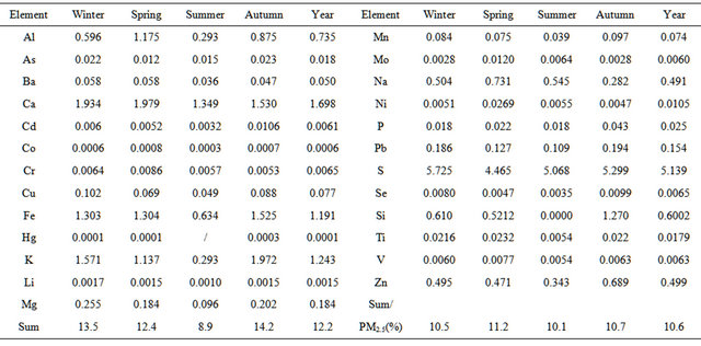
Table 3. Enrichment factors of 24 elements in PM2.5 samples.
(sulfate, SO2) and (nitrate, NO2) in this campaign. On molar basis, sulfate accounted for 10% - 30% of total sulfur in breathing zones, and nitrate accounted for 1% - 20% of total oxidized nitrogen during this study. Thus, seasonal variations of ionic concentrations may also result from changes in relative humidity near sampling sites during this campaign.
Also shown in Figure 2 is the ratio of cation/anion in PM2.5 samples. The ratio ranged 1.0 - 1.6 with the average of 1.2 in breathing zones, and was 1.1 at a routine automatic monitoring station. Thus, organic anions might be present significantly during the campaign.
As sulfate concentration was measured concurrently with the concentration of elemental sulfur in this study, a comparison between the two concentrations may offer unique insights into the existence of organic sulfur compounds. During this study, the average concentration of S was 5.14 µg∙m−3, and that of sulfate 14.5 µg∙m−3; thus, it is likely that organic sulfur concentration was minor (~0.3 µg∙S∙m−3) compared with inorganic sulfur.
3.4. Carbon Distribution
Concentrations of total carbon (TC), organic carbon (OC), and elemental carbon (EC) in PM2.5 were measured to be 32, 21, and 11 µg∙m−3, respectively, during the campaign. Total carbon accounted for 28% of PM2.5 concentration in the breathing zones.
Figure 3 shows seasonal concentrations of OC and EC in PM2.5 and corresponding ratio of OC/EC at various stations. It is shown that seasonal TC and OC concentrations peaked in fall and showed minimal values in summer, while EC showed much smaller seasonality; thus, OC drove the seasonal trend of TC in the campaign. The seasonal ratio of OC/EC showed minimum value in summer, and peaked in fall in breathing zones. At the suburban background station (5 m AGL), the ratio of OC/EC peaked in summer while the TC concentration was the lowest.
The correlation between OC and EC concentrations is often used to determine whether they come from the
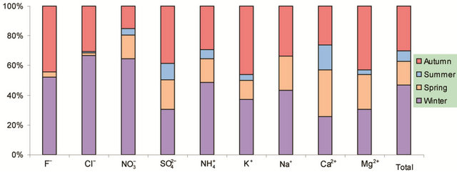
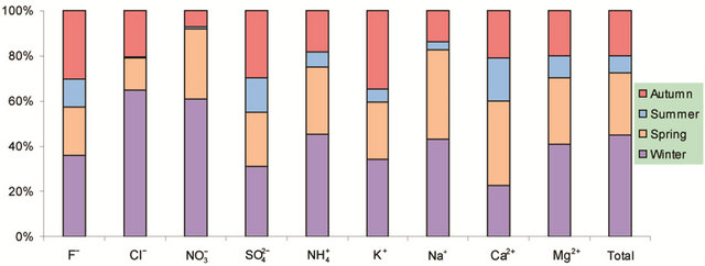
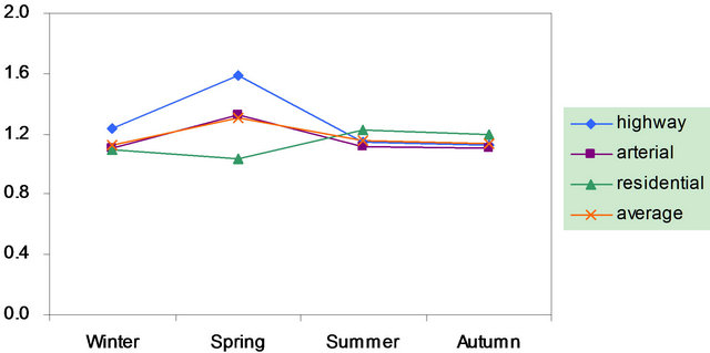
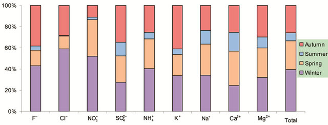
Figure 2. Seasonal variations of soluble ions in PM2.5 samples. Top left: highway; top right: arterial; bottom left: residential; bottom right: C/A ratios.
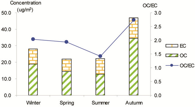
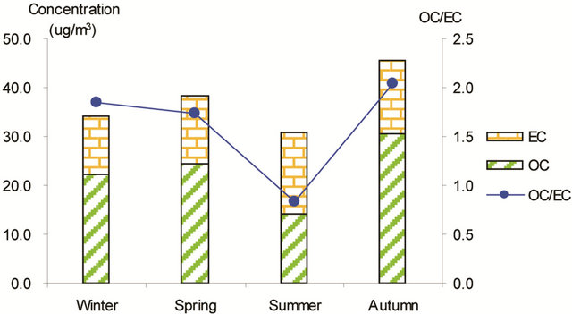

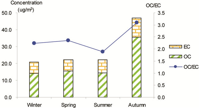
Figure 3. Seasonal average concentrations of OC and EC and their ratios in PM2.5 samples. Top left: arterial; top right: highway; bottom left-residential road, bottom right: residential areas.
same origin [30-32], as OC may be either produced by gas to particle conversion processes or directly emitted, while EC is usually directly emitted from fossil fuel combustion and biomass burning [33]. Figure 4 shows seasonal scatterplots of OC versus EC measurements in breathing zones during the campaign. It is shown that OC and EC concentrations were highly correlated in winter (R2 = 0.85, slope = 2.0) and spring (R2 = 0.78, slope = 1.7). In summer and especially in fall, the OC concentration was poorly correlated with EC. In summer, data points split into two groups: one with a slope about 2, and the other with a slope about 0.5. In fall, data points may be bracketed by two lines with the ratio of OC/EC equals 2 and 4, respectively. The higher ratio of OC/EC was likely due to photochemical aging, and the lower ratio of OC/EC was likely due to fresh emissions or due
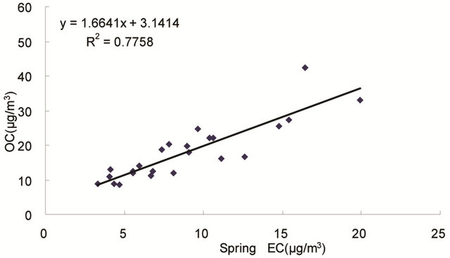

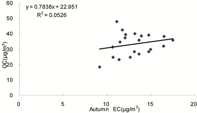

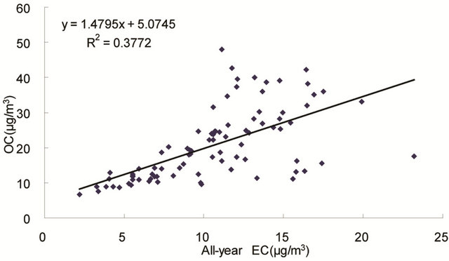
Figure 4. Scatter-plots of PM2.5 OC and EC concentrations in four seasons.
to frequent rainfall that might remove more OC than EC from the air besides other factors.
Secondary organic aerosols are important for many scientific reasons, and consist of many compounds which are only partly identified [34]. Yu et al. [35] for the first time estimated the spatial distribution of secondary organic carbon (SOC) over USA in summer, 1999. During the study period, major sources of primary OC were agricultural burning, soil dust, paved road dust and non-road diesel, while major sources of EC were non-road diesel, on-road heavy-duty diesel vehicle, agricultural burning and jet fuel combustion in USA. They showed that, on seasonal scale, modeled ratio of primary (OC/EC) changed significantly at specific locations, with values ranging from 0.8 to 3.5 at stations due to various combinations of emission sources. Meanwhile, the contribution of SOC to total OC ranged 50% - 80% based on combined analyses of observational and modeled data. In a subsequent study employing US EPA CMAQ, simulated seasonal average ratio of primary (OC/EC) over various regions of USA ranged from 2.0 to 3.6, and estimated that SOC contributed less to total OC in 2001 compared with that in 1999 [36,37].
While it is elegant to estimate SOC from modeled ratio of primary (OC/EC) and measured EC, using measured EC as a tracer for primary OC may provide a preliminary estimate for measured SOC, with all possible uncertainties embedded in field data [35]. Using empirical formula (F1) below, SOC may be estimated from OC, EC, and the minimum ratio of OC/EC during a period.
 (F1)
(F1)
On seasonal basis, (OC/EC)min ranged 0.71 - 2.3 in this campaign, and SOC was estimated to range from 1.2 to 9.6 µg∙m−3 in breathing zones using formula (F1).
4. Conclusions
In this work, we observed significant temporal and geographical variations in PM pollution over a subtropical metropolitan area through a multi-institutional field campaign in Hangzhou, China. During the campaign, we captured serious PM2.5 pollutions in the breathing zone of the scenic city in all seasons. A number of toxic metals were highly enriched in the breathing zone due to anthropogenic activities. The annual average concentration of PM2.5 ranged from 106 to 131 µg∙m−3 in the metropolitan breathing zones, which were 40% - 70% higher than at typical ambient stations. Speciation of PM2.5 was carried out for 25 elements using instrumental analyses by ICP, ICP-MS, and AFS, for 9 soluble ions using IC, and for (TC, OC, EC) using a thermo-photometric method.
A number of toxic metals were highly enriched in the breathing zone due to anthropogenic activities. Elemental analyses revealed significant presences of toxic heavy metals (Hg, Cd, Cr, Pb, As) in PM2.5 and that, among 25 detected elements, (S, Ca, K, Fe) showed concentrations larger than 1.0 µg∙m−3. Enrichment factor analysis revealed that (Cd, Se, S, Mo, Zn, Pb, Cu, As) in PM2.5 were dominated by anthropogenic sources. Nine soluble ions detected during the campaign contributed 42 µg∙m−3 to PM2.5 concentration on average, and three secondary inorganic ions ( ,
,  ,
, ) accounted for 85% of total ionic concentration. Nitrate concentration was close to and occasionally exceeded sulfate concentration during the campaign, which reflects rising vehicle activities. Molar ratios of sulfate/(total sulfur) and nitrate/(total oxidized nitrogen) frequently exceeded 10%, which suggests significant effects of photochemical reactions on PM2.5 pollution in the breathing zones.
The average total carbon concentration was 32 µg∙m−3, and the average ratio of OC/EC was 2. During the campaign, seasonal variation of TC was dominated by OC, and both concentrations peaked in fall and were low in summer. The EC concentration showed little seasonality, and OC was well correlated with EC in winter and spring. Secondary organic carbon was estimated to contribute 1.2 - 9.6 µg∙m−3 to PM2.5 concentration in the breathing zones. Comparison of concurrent measurements of sulfur element and sulfate suggests that the average concentration of organic sulfur (0.3 µg∙S∙m−3) in PM2.5 samples was relatively small compared with inorganic sulfur during the campaign.
5. Declaration
This work has been reviewed by staff at Zhejiang Environmental Protection Agency, China, and has been approved for publication. Approval does not signify the endorsement of commercial products mentioned in this article, and opinions in this article are solely those of authors.
6. Acknowledgements
We thank Dr. Shaocai Yu at US EPA, Dr. Jinyou Liang at Zhejiang University, and anonymous reviewers for having critically reviewed this article. This work was partly supported by Hangzhou Bureau of Science and Technology (Grant 20091133B15), China.
REFERENCES
- K. Huang, G. Zhuang, Y. Lin, J. S. Fu, Q. Wang, T. Liu, R. Zhang, Y. Jiang, C. Deng, Q. Fu, N. C. Hsu and B. Cao, “Typical Types and Formation Mechanisms of Haze in an Eastern Asia Megacity, Shanghai,” Atmospheric Chemistry and Physics, Vol. 12, No. 1, 2012, pp. 105- 124. doi:10.5194/acp-12-105-2012
- B. Hou, G. Zhuang, R. Zhang, T. Liu, Z. Guo and Y. Chen, “The Implication of Carbonaceous Aerosol to the Formation of Haze: Revealed from the Characteristics and Sources of OC/EC over a Mega-City in China,” Journal of Hazardous Materials, Vol. 190, No. 1-3, 2011, pp. 529-536. doi:10.1016/j.jhazmat.2011.03.072
- X. N. Ye, Z. Ma, J. C. Zhang, H. H. Du, J. M. Chen, H. Chen, X. Yang, W. Gao and F. H. Geng, “Important Role of Ammonia on Haze Formation in Shanghai,” Environmental Research Letters, Vol. 6, No. 2, 2011, p. 024019. doi:10.1088/1748-9326/6/2/024019
- A. P. K. Tai, L. J. Mickley and D. J. Jacob, “Correlations between Fine Particulate Matter (PM2.5) and Meteorological Variables in the United States: Implications for the Sensitivity of PM2.5 to Climate Change,” Atmospheric Environment, Vol. 44, No. 32, 2010, pp. 3976-3984. doi:10.1016/j.atmosenv.2010.06.060
- J. Lewtas, “Air Pollution Combustion Emissions: Characterization of Causative Agents and Mechanisms Associated with Cancer, Reproductive, and Cardiovascular Effects,” Mutation Research, Vol. 636, No. 1-3, 2007, pp. 95-133. doi:10.1016/j.mrrev.2007.08.003
- D. S. Grass, J. M. Ross, F. Family, J. Barbour, H. James Simpson, D. Coulibaly, J. Hernandez, Y. Chen, V. Slavkovich, Y. Li, J. Graziano, R. M. Santella, P. Brandt-Rauf and S. N. Chillrud, “Airborne Particulate Metals in the New York City Subway: A Pilot Study to Assess the Potential for Health Impacts,” Environmental Research, Vol. 110, No. 1, 2010, pp. 1-11. doi:10.1016/j.envres.2009.10.006
- A. Zanobetti and J. Schwartz, “The Effect of Fine and Coarse Particulate Air Pollution on Mortality: A National Analysis,” Environmental Health Perspectives, Vol. 117, No. 6, 2009, pp. 898-903. doi:10.1289/ehp.0800108
- J. Feng and W. Yang, “Effects of Particulate Air Pollution on Cardiovascular Health: A Population Health Risk Assessment,” Plos One, Vol. 7, No. 3, 2012, p. e33385. doi:10.1371/journal.pone.0033385
- Z. Q. Lin, Z. G. Xi, D. F. Yang, F. H. Chao, H. S. Zhang, W. Zhang, H. L. Liu, Z. M. Yang and R. B. Sun, “Oxidative Damage to Lung Tissue and Peripheral Blood in Endotracheal PM2.5-Treated Rats,” Biomedical and Environmental Sciences, Vol. 22, No. 3, 2009, pp. 223-228. doi:10.1016/S0895-3988(09)60049-0
- Y. Wei, I. K. Han, M. Hu, M. Shao, J. J. Zhang and X. Tang, “Personal Exposure to Particulate PAHs and Anthraquinone and Oxidative DNA Damages in Humans,” Chemosphere, Vol. 81, No. 10, 2010, pp. 1280-1285. doi:10.1016/j.chemosphere.2010.08.055
- Y. J. Lee, Y. W. Lim, J. Y. Yang, C. S. Kim, Y. C. Shin and D. C. Shin, “Evaluating the PM Damage Cost Due to Urban Air Pollution and Vehicle Emissions in Seoul, Korea,” Journal of Environmental Management, Vol. 92, No. 3, 2011, pp. 603-609. doi:10.1016/j.jenvman.2010.09.028
- N. Z. Muller and R. Mendelsohn, “Measuring the Damages of Air Pollution in the United States,” Journal of Environmental Economics and Management, Vol. 54, No. 1, 2007, pp. 1-14. doi:10.1016/j.jeem.2006.12.002
- M. Sillanpaa, A. Frey, R. Hillamo, A. S. Pennanen and R. O. Salonen, “Organic, Elemental and Inorganic Carbon in Particulate Matter of Six Urban Environments in Europe,” Atmospheric Chemistry and Physics, Vol. 5, No. 11, 2005, pp. 2869-2879.
- Y. F. Lam, J. S. Fu, S. Wu and L. J. Mickley, “Impacts of Future Climate Change and Effects of Biogenic Emissions on Surface Ozone and Particulate Matter Concentrations in the United States,” Atmospheric Chemistry and Physics, Vol. 11, No. 10, 2011, pp. 4789-4806. doi:10.5194/acp-11-4789-2011
- X. Y. Zhang, Y. Q. Wang, T. Niu, X. C. Zhang, S. L. Gong, Y. M. Zhang and J. Y. Sun, “Atmospheric Aerosol Compositions in China: Spatial/Temporal Variability, Chemical Signature, Regional Haze Distribution and Comparisons with Global Aerosols,” Atmospheric Chemistry and Physics, Vol. 12, No. 2, 2012, pp. 779-799. doi:10.5194/acp-12-779-2012
- D. McCubbin, “Health Benefits of Alternative PM2.5 Standards,” American Lung Association, Clean Air Task Force, Earthjustice, Washington, 2011. http://www.earthjustice.org/sites/default/files/Health-Benefits-Alternative-PM2.5-Standards.pdf.
- X. Li, L. Wang, Y. Wang, T. Wen, Y. Yang, Y. Zhao and Y. Wang, “Chemical Composition and Size Distribution of Airborne Particulate Matters in Beijing during the 2008 Olympics,” Atmospheric Environment, Vol. 50, 2012, pp. 278-286. doi:10.1016/j.atmosenv.2011.12.021
- S.-C. Lai, S.-C. Zou, J.-J. Cao, S.-C. Lee and K.-F. Ho, “Characterizing Ionic Species in PM2.5 and PM10 in Four Pearl River Delta Cities, South China,” Journal of Environmental Sciences, Vol. 19, No. 8, 2007, pp. 939-947. doi:10.1016/S1001-0742(07)60155-7
- D. Houthuijs, O. Breugelmans, G. Hoek, E. Vaskovi, E. Mihalikova, J. S. Pastuszka, V. Jirik, S. Sachelarescu, D. Lolova, K. Meliefste, E. Uzunova, C. Marinescu, J. Volf, F. de Leeuw, H. van de Wiel, T. Fletcher, E. Lebret and B. Brunekreef, “PM10 and PM2.5 Concentrations in Central and Eastern Europe: Results from the Cesar Study,” Atmospheric Environment, Vol. 35, No. 15, 2001, pp. 2757- 2771.
- F. Yang, J. Tan, Q. Zhao, Z. Du, K. He, Y. Ma, F. Duan, G. Chen and Q. Zhao, “Characteristics of PM2.5 Speciation in Representative Megacities and across China,” Atmospheric Chemistry and Physics, Vol. 11, No. 11, 2011, pp. 5207-5219.
- J. C. Chow, J. G. Watson, L. C. Pritchett, W. R. Pierson, C. A. Frazier and R. G. Purcell, “The DRI Thermal Optical Reflectance Carbon Analysis System—Description, Evaluation and Applications in United-States Air-Quality Studies,” Atmospheric Environment Part A—General Topics, Vol. 27, No. 8, 1993, pp. 1185-1201.
- J. G. Watson, J. C. Chow, D. H. Lowenthal, L. C. Pritchett, C. A. Frazier, G. R. Neuroth and R. Robbins, “Differences in the Carbon Composition of Source Profiles for Diesel-Powered and Gasoline-Powered Vehicles,” Atmospheric Environment, Vol. 28, No. 15, 1994, pp. 2493- 2505. doi:10.1016/1352-2310(94)90400-6
- K. F. Ho, S. C. Lee, J. C. Chow and J. G. Watson, “Characterization of PM10 and PM2.5 Source Profiles for Fugitive Dust in Hong Kong,” Atmospheric Environment, Vol. 37, No. 8, 2003, pp. 1023-1032. doi:10.1016/S1352-2310(02)01028-2
- J. C. Chow, J. G. Watson, L. W. A. Chen, W. P. Arnott and H. Moosmuller, “Equivalence of Elemental Carbon by Thermal/Optical Reflectance and Transmittance with Different Temperature Protocols,” Environmental Science & Technology, Vol. 38, No. 16, 2004, pp. 4414-4422. doi:10.1021/es034936u
- J. C. Chow, J. G. Watson, L. W. A. Chen, G. ParedesMiranda, M. C. O. Chang, D. Trimble, K. K. Fung, H. Zhang and J. Z. Yu, “Refining Temperature Measures in Thermal/Optical Carbon Analysis,” Atmospheric Chemistry and Physics, Vol. 5, No. 11, 2005, pp. 2961-2972.
- H. S. El-Zanan, D. H. Lowenthal, B. Zielinska, J. C. Chow and N. Kumar, “Determination of the Organic Aerosol Mass to Organic Carbon Ratio in IMPROVE Samples,” Chemosphere, Vol. 60, No. 4, 2005, pp. 485-496. doi:10.1016/j.chemosphere.2005.01.005
- Y. M. Han, J. J. Cao, J. C. Chow, J. G. Watson, Z. S. An, Z. D. Jin, K. C. Fung and S. X. Liu, “Evaluation of the Thermal/Optical Reflectance Method FOR Discrimination between Charand Soot-EC,” Chemosphere, Vol. 69, No. 4, 2007, pp. 569-574. doi:10.1016/j.chemosphere.2007.03.024
- H. S. El-Zanan, B. Zielinska, L. R. Mazzoleni and D. A. Hansen, “Analytical Determination of the Aerosol Organic Mass-To-Organic Carbon Ratio,” Journal of the Air & Waste Management Association, Vol. 59, No. 1, 2009, pp. 58-69. doi:10.3155/1047-3289.59.1.58
- X. D. Feng, Z. Dang and W. L. Huang, “Pollution Level and Chemical Speciation of Heavy Metals in Pm2.5 during Autumn in Guangzhou City,” Huan Jing Ke Xue, Vol. 29, No. 3, 2008, pp. 569-575.
- B. J. Turpin and J. J. Huntzicker, “Identification of Secondary Organic Aerosol Episodes and Quantitation of Primary and Secondary Organic Aerosol Concentrations during SCAQS,” Atmospheric Environment, Vol. 29, No. 23, 1995, pp. 3527-3544. doi:10.1016/1352-2310(94)00276-Q
- R. Strader, F. Lurmann and S. N. Pandis, “Evaluation of Secondary Organic Aerosol Formation in Winter,” Atmospheric Environment, Vol. 33, No. 29, 1999, pp. 4849- 4863. doi:10.1016/S1352-2310(99)00310-6
- H. A. Gray, G. R. Cass, J. J. Huntzicker, E. K. Heyerdahl and J. A. Rau, “Characteristics of Atmospheric Organic and Elemental Carbon Particle Concentrations in Los Angeles,” Environmental Science & Technology, Vol. 20, No. 6, 1986, pp. 580-589. doi:10.1021/es00148a006
- J. C. Cabada, S. N. Pandis, R. Subramanian, A. L. Robinson, A. Polidori and B. Turpin, “Estimating the Secondary Organic Aerosol Contribution to PM2.5 Using the EC Tracer Method,” Aerosol Science and Technology, Vol. 38, Supplement 1, 2004, pp. 140-155.
- S. C. Yu, “Role of Organic Acids (Formic, Acetic, Pyruvic and Oxalic) in the Formation of Cloud Condensation Nuclei (CCN): A Review,” Atmospheric Research, Vol. 53, No. 4, 2000, pp. 185-217. doi:10.1016/S0169-8095(00)00037-5
- S. C. Yu, R. L. Dennis, P. V. Bhave and B. K. Eder, “Primary and Secondary Organic Aerosols over the United States: Estimates on the Basis of Observed Organic Carbon (OC) and Elemental Carbon (EC), and Air Quality Modeled Primary OC/EC ratios,” Atmospheric Environment, Vol. 38, No. 31, 2004, pp. 5257-5268. doi:10.1016/j.atmosenv.2004.02.064
- S. C. Yu, R. Mathur, K. Schere, D. W. Kang, J. Pleim, J. Young, D. Tong, G. Pouliot, S. A. McKeen and S. T. Rao, “Evaluation of Real-Time PM2.5 Forecasts and Process Analysis for PM2.5 Formation over the Eastern United States Using the Eta-CMAQ Forecast Model during the 2004 ICARTT Study,” Journal of Geophysical ResearchAtmospheres, Vol. 113, No. D6, 2008, Article No. D06204. doi:10.1029/2007JD009226
- S. Yu, P. V. Bhave, R. L. Dennis and R. Mathur, “Seasonal and Regional Variations of Primary and Secondary Organic Aerosols over the Continental United States: SemiEmpirical Estimates and Model Evaluation,” Environmental Science & Technology, Vol. 41, No. 13, 2007, pp. 4690-4697. doi:10.1021/es061535g
NOTES
*Corresponding author.