International Journal of Geosciences
Vol.4 No.2(2013), Article ID:29370,10 pages DOI:10.4236/ijg.2013.42037
Luminous Shapes with Unusual Motions as Potential Predictors of Earthquakes: A Historical Summary of the Validity and Application of the Tectonic Strain Theory
1Laurentian University, Sudbury, Canada
2Tijeras, New Mexico, USA
Email: mpersinger@laurentian.ca, shakyace@yahoo.com
Received December 15, 2012; revised January 16, 2013; accepted February 15, 2013
Keywords: Tectonic Strain; Luminous Phenomena; Earthquake Forecasting; Hydrological Loads
ABSTRACT
For centuries and on every continent discrete shapes of lights with unusual motions have preceded earthquakes. The numbers of these lights per interval within a region have been strongly correlated with the amount of seismic energy subsequently released within that region. These temporal intervals range between 3 months and 6 months for areas more than 500 km in radius and less than a month for smaller radii. Other analyses have shown that the same tectonic strain associated with earthquakes is also associated with the display of luminous events before those earthquakes. This strain can be precipitated by injections of fluids into the crust, natural changes in hydrological loads on rivers, or, purposeful displacement of water into reservoirs. The strengths of the associations are sufficient to allow modest forecasting of earthquakes within the boundaries of the region and the temporal interval of analysis. More accurate utilization of these phenomena as prognosticators of specific earthquakes will require a re-evaluation of the manner by which these data are systematically recorded and interpreted.
1. Introduction
The forecasting of natural phenomena has often begun with the isolation of stimuli that systematically preceded the occurrence of the phenomenon. Unless a 1:1 relationship exists between a class of predictors and a class of events and this relationship is within the temporal limitations of human perception, the association may be difficult to discern. If significant time separates the predictor and the event and these durations are variable, casual attention may not have the resolution to extract the systematic relationship from the background of observational noise. One example of this type of relationship is between the numbers of reports of odd, luminous events and the occurrence of earthquakes days to months later. Recently we [1] found that ground photon emissions increased about two weeks before large M9.0 earthquakes. However there has been a long history of unusual seismic antecedents [1]. Here we review the evidence for discrete localized luminous phenomena that precede the range in earthquake magnitudes days to months before the regional event.
An example of the temporal contiguity between brief, discrete, lights in the sky (or geoatmospheric lights) and earthquakes was reported by St-Laurent [2]. However the first recorded sightings of earthquake lights dates from 373 BCE in Greece. Although the explanations for the phenomena have changed over time and within different cultures, the details have been remarkably consistent. For example “pyramids of a fiery red colour” and “elliptical corona of amazing brightness” were observed about two weeks before an earthquake that was felt in London, England in 1749-1750.
During the early twentieth century, luminous phenomena, occurring between a few km to several hundreds of km from epicentres, were reported by Italian and German seismologists. Milne [3] reviewed the significant work published in 1910 of Ignazio Galli [4] who categorized the luminous phenomena accompanying earthquakes into four categories each with several subcategories. In 1931 the Japanese researcher Terada [5] summarized the luminous phenomena observed in the sky or on the ground before, during, and after the time of severe shocks in Japan. The categories, which were very similar to those of Galli, included luminous masses, fireballs, bright funnels, beams of fire, and flames.
For example before an earthquake in Japan during 1672, a fire ball resembling a paper-lantern was seen; before the Tossa earthquake in 1698, a number of fiery wheels were seen flying in different directions. Before the 26 November, 1930 earthquake in the Idu district of Japan, luminous phenomena were seen within a radius of about 50 km from the epicentre. During the 24 hr before the seismic event a spherical luminous body was seen moving at considerable speed. Near the epicentral districts ball, trumpet, funnel-shaped lights were seen. When the earthquake was at its height, a straight row of round masses of light were seen; each body seemed to be revolving on its own axis [5].
The global nature of luminous phenomena and their relationship to rock fracture was revisited in 1986 by Derr [6]. There have been many hypotheses to explain these phenomena that range from nuclear-like processes, similar to ball lightning [7], to piezoelectric manifestations from moving pressure gradients [8]. Parametric instability of water droplets in an electric field has been suggested as one mechanism [9] exacerbated by pore fluid pressure in anisotropic rocks [10] to produce luminous phenomena with life times in the order of 10 to 100 s. Plasma fireballs with durations of several minutes were produced reliably by microwave (2.45 GHz), kW power oscillators in the laboratory by Ohtsuki and Ofuruton [11].
2. Luminous Events Days to Months before Seismic Events
For more than 30 years we have been developing the Tectonic Strain Theory or TST [12-15] to explain a specific class of luminous phenomena that have been considered “strange”, primarily because the physical mechanisms are not clear and there is minimum consensus by the scientific community about their significance. Usually they are classified under anomalous or peripheral categories that include “unidentified” events or objects. The TST states that strain fields induced within rock by tectonic stresses generate electromagnetic phenomena and include the visible wavelengths. The specific types of visible phenomena are a function of the rate of increase of the tectonic strain, its space-time metrics (tensor) and the geochemistry of the crustal material within which the strain is induced. Piezoelectric capacities of the local rock are the central but not the only contributor to the occurrence of luminosities. The phenomena are very similar to earthquake lights, which occur during or immediately before earthquakes, except the emergence occurs weeks to months before the key seismic event. The majority of these phenomena occur along stress release regions such as fault lines. A similar concept was developed by Devereux [16].
These luminous phenomena are usually reported as spherical, oblate, or triangular. The colors, which we assume reflect intrinsic temperature, are usually white, red, or blue. They show all of the characteristics of earthquake lights except they can occur days to months (1 Megasec to 10 Megasec) before earthquakes. Some of these phenomena display multicolors or subsets of colors that we have hypothesized could reflect different regions of temperature within the event. Like most of the earthquake lights reported in previous centuries, these luminous phenomena are often “reddish”. When the phenomena can be observed during the day they may appear darker than the background sky but still maintain the shapes of triangles, pyramids, circles or ellipses. This can be associated with the perceptual illusion of a discrete object. We suspect this “darkness” would be analogous to the perceptions of the solar surface where cooler regions, such as sunspots, appear “black” [17].
Because the phenomena are associated with strain within the earth’s crust, we have also predicted that some of these day-time events may appear “metallic”. Reflectance, sufficient to be perceived as metallic for a sphere of 1 m wide, would require only a few gm of liquefied metal if the stable surface thickness was about 5 µm [17]. These materials have been observed to be “precipitated” if the phenomenon changed state or contacted the ground. Interestingly, the most common constituents of “residua” found in these rare events are silicates, aluminium, iron, and magnesium, the most abundant elements of the earth’s crust.
The life times of stationary luminous displays generally range from 10 to 100 sec. Their spatial parameters range between 1 m to several meters. The power output has been estimated, primarily from photographic evidence and may exceed the kilowatt range. Close proximity to some but not all of the larger phenomena have been associated with disruptions of electrical systems and interference with the operation of automobile engines (but not diesels). Radon gas, that is known to be released before and during some earthquakes, has been recorded on the ground especially if the phenomenon was seen to emerge from the surface.
In some instances close proximity to these luminous phenomena by human beings or animals has been associated with skin burns and unconsciousness. The syndromes that follow these episodes are congruent with the consequence of induction of electrical currents within brain tissue sufficient to induce unconsciousness, disrupt memory consolidation (amnesia), and, affect the accurate reconstruction of events. We suspect that mortality has occurred but the predicted post-mortem results would have been difficult to differentiate from electrocution by a lightning strike [18].
To date the mechanisms by which the luminous phenomena are generated and maintained for several tens of seconds are not completely clear. The processes maintaining the spatial and temporal integrity of ball lightning may have equivalents for the luminous phenomena preceding earthquakes. The factors determining the parameters for the major range in the radii of the phenomena are also not clear. However we suspect the historical persistence in the width of these phenomena may reflect the upper and lower boundaries of the “quanta” of energy, derived from the tectonic strain, which generates the individual event. One metaphor is bubble formation in air. Although there is a normal distribution in the lifetimes and the width of the bubbles with each display of energy (air moving through a closed boundary within which a liquid is suspended), the absolute boundaries of the radii are constrained by the physical properties of the materials from which they are generated.
In general the movements of these phenomena through space reflect the local topography. These globular phenomena tend to follow local fault lines [17]. Stationary positions occur near the apices of hills, on the tops of trees, near power lines, or over any conductor such as radio transmitter towers. Very fast velocities are displayed when the phenomena move quickly towards the upper troposphere. Although human estimates suggest extraordinary speeds, the more reliable measurements indicate velocities typical of point tidal forces moving along a fault line, e.g., about 1,700 km/hr.
The central theme of the Tectonic Strain Theory is that most luminous displays are generated by the same geophysical processes that produce earthquakes. As the strain slowly accumulates within a susceptible region luminous events are produced intermittently for weeks to months. When the strain achieves a critical value, an earthquake occurs. Although luminous phenomena precede earthquakes they do not cause earthquakes. Instead, both are caused by the same normal geophysical process: transient tectonic strain from local and far-field stresses [13].
We have selected the term strain rather than tectonic stress or earth stress because our model and results indicate luminous phenomena are consequences of processes (and the temporal derivatives of these processes) induced within the earth’s crust by primarily compression stresses. Several of our quantitative studies have shown that the rate of change in the strain (or derivative) may be a very large contributory factor to the generation of luminous phenomena before an earthquake. Partial correlation analyses, that allow identification of shared sources of numerical variance, have also indicated that the telluric currents within a susceptible region following sudden, intense increases in global geomagnetic activity can also facilitate the numbers of luminous events [19].
If one assumes that tectonic strain is the primary cause of luminous phenomena and earthquakes, then one might also predict that both would occur within more or less the same regions. This prediction has been supported empirically [15]. Some areas would have histories of only a few reports of luminous phenomena while other areas would be the loci of such copious numbers of reports they would not be recorded because they would be routine and even mundane. The Tectonic Strain Theory predicts there should be strong positive relationships between the numbers of luminous events and the numbers of earthquakes or the total amount of energy released by the earthquakes.
However the accurate prediction of earthquakes from the numbers of luminous phenomena would require the isolation of the optimal increment of spaces to be compared and the optimal increments of times by which these comparisons are analyzed. The primary data sources for our analyses were from national and local registries for “unidentified flying objects”, “anomalous air phenomena” and observation posts (for monitoring forested areas for fires). Categories selected involved luminous phenomena displaying unusual colors and undulating or erratic movements that were persistent for several tens of seconds. Luminous phenomena that were linear in motion, associated with obvious air or satellite traffic, or from questionable reporting were not included. In fact the numbers of events from the latter category were employed as “comparator” or control samples and were never strongly associated with the subsequent increase in seismicity within the region. Only the luminosities with characteristics similar to those associated with actual earthquake lightning were significantly correlated with the release of seismic energy weeks to months later.
We have found the optimal area required to demonstrate a robust relationship between the occurrence of luminous phenomena and subsequent earthquakes within the area is influenced by the crustal structure. This repeated observation would be consistent with our assumption that most luminous phenomena are related to regional processes rather than to the very local events where they are observed. For crustal concavities, such as the Uinta Basin in Utah [20] and the San Francisco Basin in California [21], the optimal cross-section area may be in the order of 10,000 square km. This would involve a radius of about 50 km. For larger tectonic areas, such as the New Madrid system, the diameter would be in the order of 500 km while for the larger homogeneous tectonic areas, such as the central USA and central southern Canada, the diameter could exceed 1000 km. This would mean that the recording of luminous events within the appropriate areas would be essential to reflect the tectonic strain, and hence the earthquake probability, within that area.
We have also found the temporal increment that is optimal to predict the relationship between numbers of luminous phenomena in the area and the numbers of earthquakes is more typical of the life times of geophysical processes. Seismologists have known for decades that the increment of time employed to predict seismic events is directly related to accuracy. Temporal increments of analyses that involve decades generate more accurate forecasts of the occurrence of a strong earthquake. Accuracy, when increments of days or even months are employed, decreases almost exponentially. The relationship between seismic energy release in general and the occurrence of luminous phenomena in small areas, such as the New Mexico and Colorado Rift area [22], is visually obvious where the data for both are plotted over time as shown in Figure 1 for the years 1947 through 1971.
In general, we have found that the strengths of the association between luminous phenomena and the subsequent numbers of earthquakes or the release of seismic energy, which range from Pearson rs of about 0.7 to 0.8, are greatest when the data are analyzed as successive 3 month or 6 month increments. This statement is particularly accurate for the larger areas involving several millions of square kms. Figure 2 shows the total numbers of luminous events (GLP) per interval (successive, fixed six month intervals) within the states surround the New Madrid area for the years 1945 through 1977. Usually, for six month intervals over large areas, the numbers of luminous events increase during the interval before increases in the release of seismic energy.
For smaller regions, such as the basins, day-to-day variations in geomagnetic activity, seasonal variations in hydraulic loads (from above average seasonal rain falls) or the results of cultural demands for reservoirs, lakes, and rivers, are important contributors to the prediction of both luminous phenomena and earthquakes. For example the peak in numbers of luminous events within 320 km of the centroid of the Mississippi River System is about four months after the seasonal peaks in the river level [23]. As can be seen in Figure 3, the numbers of specific luminous phenomena (closed circles), that were similar
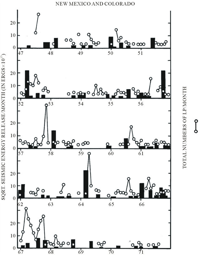
Figure 1. Square root of the seismic energy release (bars) per month and the total numbers of luminous phenomena (LP) reported per month (open circles) within New Mexico and Colorado.

Figure 2. Scattergram for the square root of the numbers of Luminous Phenomena (GLP) reported per 6-month interval and the square root of the sum of the seismic energy release during the following 6-month interval for the sector involving the states surround the New Madrid region in the central USA.
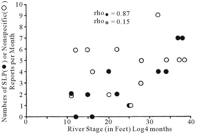
Figure 3. Correlation between numbers of luminous events (closed circles) and the stage of the Mississippi River four months previously. Open circles reflect the correlation with non-specific lights.
to traditional earthquake lights but classified as “unidentified flying or aerial objects”, were correlated strongly (rho = 0.87) with the river stage (in feet) four months previously. As comparisons, control cases (open circles), reports of lights typical of passing airplanes and streaks of lights (meteors), were not significantly correlated (rho = 0.15) with antecedent river levels.
Correlational analyses are replete with the recondite role of third variables (such as tectonic strain) that produce both phenomena as well as confounding variables that may reflect the operation of epiphenomena. Whenever possible, an experiment is the most optimal method to determine causality. Considering the energy requirements and both the spatial and temporal scale within which the relationship between numbers of luminous phenomena and seismic activity operate such experiments would appear impossible.
However, the results of large scale man-made efforts can be considered a quasi-experimental support for the Tectonic Strain Theory. One example might have been the diversion of the water in the Aral Sea and the luminous displays in Tashkent, Ubekistan during the 1960s. We suspect that close examination of the technical literature would reveal frequent incidences between injections of large volumes of fluid within “impervious rock vaults” such as mines and caverns and the production of tectonic strain and luminosities. Hydroseismicity has been long suspected to be involved centrally with intraplate earthquakes [24] because of hydrolytic weakening of minerals that leads to structural weakening. This change results in more diffuse distribution of epicentres that would be (according to the TST) reflected in a diffuse distribution of the reports of luminous phenomena within these clusters.
By far one of the most elegant examples of a quasi experimental design, although the a priori intention to test the hypothesis was not the motivation for the experiment, was the Derby (Colorado) events. It has been considered a classic case of induced seismicity [25]. Several hundreds of microseismic events followed within a few days to weeks after the injection of millions of gallons of fluid per month into the earth at the Rocky Mountain Arsenal near Denver. When the professionals working on the project appreciated this causal connection, the injections of the fluid were terminated for several months. When the injections were reinitiated, the numbers of local small earthquakes increased conspicuously again.
We employed this effectively a-b-a-b-a design, where “b” was the injection of fluid and “a” was the non-injection (normal) condition to discern the quantitative relationship between the numbers of luminous events, volume of fluid injected into the crust, and the numbers of earthquakes. Even casual inspection of the data graphically indicated that the numbers of luminous events were associated with the periods and the amount of fluid injection and the numbers of earthquakes [26]. The raw data are shown in Figure 4.
Zero order correlations indicated significant positive relationships (correlation coefficients of about 0.7) between the numbers of luminous reports, numbers of earthquakes, and the volume of fluid per month. Partial correlation analyses were employed to remove the shared variance between any of the two combinations of the three variables. The result indicated that luminous phenomena and earthquakes were significantly correlated because they both shared variance with the amount of fluid injection. We inferred that the fluid injection was a source of tectonic strain that in turn produced both the luminous phenomena and the earthquakes.
Perhaps the most surprising and compelling result of that study was the emergence of a temporal lag between
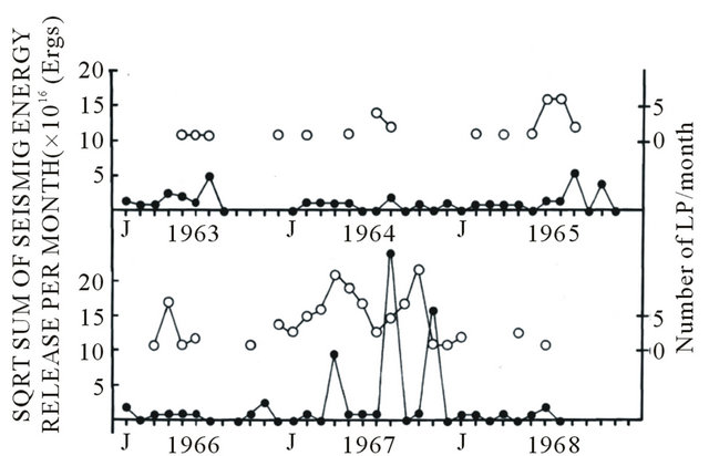
Figure 4. Square root of the seismic energy release per month (dark circles) in the Denver-Derby area of Colorado during the period injecting large amounts of fluid into the ground and the numbers of luminous phenomena (LP, open circles) reported in the area.
the amount of fluid injection per month and the numbers of luminous phenomena per month at various distances. The maximum strength correlation within 100 km of the site occurred between the numbers of luminous phenomena and the amount of fluid injected during the same month. However, for luminous phenomena occurring between 100 and 200 km from the site, the strongest correlations occurred with the amount of fluid injected two months previously. For luminous phenomena between 200 and 300 km from the site, the strongest correlation occurred with the amount of fluid injected during the previous four months. At greater distances there were no statistically significant correlations between the numbers of luminous phenomena and the amount of fluid injection, even with lags of up to 10 months. We reasoned that if luminous phenomena reflect tectonic strain, these results reflected a strain field moving away from the site at about 100 km per month or 3 km/day.
The intermittent but persistent occurrence of luminous phenomena within a geological basin within which fluid has been injected is not unique to the Rocky Mountain Arsenal. The Marfa Lights in Texas are adjacent to oil fields where, until about 1950, 80 millions of gallons of water were injected per day to help extract crude petroleum. Increased seismic activity and antecedent luminous displays appear to have been related also to petroleum production and water-flood projects near Kermit, Texas.
The possibility that the types of strain fields we predict are generating luminous displays preceding earthquakes could be aseismically propagating hydrological pulses received strong support when we evaluated other sites. We carefully analyzed areas where large amounts of fluids had been injected into underground vaults, man-made or natural, over several years. For example in addition to the 70 million gallons of fluids that were injected near Derby, Colorado, 1.6 billion gallons were injected near Rangely, Colorado. At least 840 billion liters (30 billion cubic feet) of low-level, highly acidic radioactive waste water has been deposited in ponds and wells near Hanford, Washington between 1944 and 1989. Within 100 km of these areas some of the most persistent and robust displays of luminosities have been documented [13,19].
To discern potential similarities between different regions we compared the quantitative relationship between the injection of the fluids and the numbers of luminous phenomena during the same year and each of the subsequent two years as a function of progressive radii of 100 km increments. The following sites were compared: Attica, New York (pumping brine), Rangely, Colorado (petroleum industry), Derby, Colorado (chemical products), Hanford, Washington (radioactive fluids), and the Sanford Dam, Texas (associated with the filling of Lake Meredith). In general there was a significant increase in luminous phenomena within 100 to 200 km from the sites about two years after the initiation of the injection or containment of large volumes of fluid [27].
Figure 5 shows the scattergram for the distance of major reports of luminosities (in km) as a function of time since the injections began in Attica, N.Y. If we assume that the luminosities reflected a moving strain field, then the “movement” was about 40 km/year. Given the standard error of the slope, the values could have ranged between 25 km/year and 60 km/year.
Although different areas displayed different parameters, detailed analyses indicated that the temporal lags were congruent with a diffusion process. During the first six months the successive increases in distance of the occurrence of the luminous phenomena was about 30 km
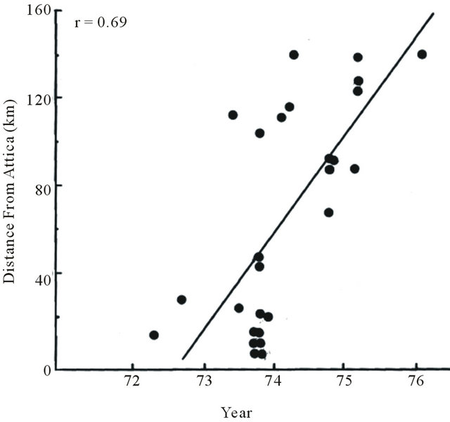
Figure 5. The relationship between the year since initiation of fluid injection and distance (in km) of all luminous phenomena within a 200 km radius from Attica over several years. r = the correlation coefficient.
per month (1 km per day). The concept of a diffusion gradient was indicated by the contemporary (same monthly interval) strong association between injection volume and numbers of luminous phenomena within 50 km of the sites. Longer, more protracted temporal lags (indicating slowing velocities of radial diffusion) between the initiation of the injections and both the occurrence and the numbers of luminous phenomena were evident as the distance increased from the injection sites.
Changes in hydraulic loads within bodies of water have been associated with the display of both luminous events and earthquakes. We have shown, by correlational analyses, that the massive display of luminous events over Zeitoun (Cairo), Egypt in the late 1960s was likely related to loads on the Aswan Dam and to subsequent seismic activity [28] near the Gulf of Suez (Ms = 6.9) in March, 1969 that caused severe damage in Egypt [29]. The possibility that hydraulic loads diverted to manmade reservoirs could generate sufficient strain to trigger large earthquakes was first appreciated with the seismicity resulting from the filling of Lake Mead behind Boulder (Hoover) Dam in the 1930s [30]. However, the September 1993 earthquake (6.1 magnitude) that killed 10,000 people in India is the most disastrous example of this phenomenon. It occurred within 15 km of a reservoir that had been filled just two years previously.
3. Accuracies of Correlations
During the last 30 years of our quantitative analyses we have found that the limiting factor for the strength of the associations between the reports of luminous events and subsequent earthquake activity has been the reports. This limitation is due to the intrinsic nature of the measurement. First, unlike seismic events there is no continuous monitoring of luminous events. Second, luminous events are local phenomena whose visibilities may be restricted to within a few km or less.
Because of their brief lifetimes and the requirement for human beings to perceive and to report them, the systematic monitoring of luminous phenomena has not occurred. We have found that as the surveillance of an area becomes more complete (such as the data from the fire lookouts near Satus Peak, Yakima, Washington before the Mt. St. Helens eruption), the strength of the association between the numbers of luminous events and the amount of energy to be released by seismic events increases markedly.
Consequently, because of the limits of the sampling of luminous phenomena, we have relied on data bases that include very large spatial areas and longer time-intervals in order to study the relationships between numbers of luminous events and subsequent release of seismic energy. Many of these data bases were collected by researchers interested in “unidentified” flying objects because most of these natural luminous phenomena coupled to tectonic strain appear to have been classified (since about 1945) by this over inclusive and heterogeneous label. However, without the enthusiasm and dedication of these researchers, despite their attributions, the data would have never been collected. Before 1945, these same or very similar phenomena also occurred before major releases of seismic energy as we have shown for both the central USA [31] and Western Europe [32]. However then they were labelled as “mysterious airships” or superstitious entities.
Obviously, the quality of the data limits both the temporal and spatial resolution of analyses. Although the correlation coefficients are still about 0.7 to 0.8 for these data bases, the intercepts for the regression lines are not zero. This means that there is a constancy of “noise”, probably erroneous reports, contained within the data. However, more than half of the variability in these reports has been associated with the later release of seismic energy within the area. In other words if the correlation is 0.8 between the release of seismic energy and a range of luminous events between 100 and 400 per temporal increment, the addition of a constant of 1000, e.g., 1100 to 1400 to the numbers of luminous events does not change the strength of the correlation or the amount of variance associated with the later release of seismic energy.
4. The Dynamics of Luminous Movement before Earthquakes
If the occurrences of luminous phenomena over more than 100 thousand sq km of surface within 1 month intervals reflect movements in strain fields, then the visualization of these changing fields would be difficult by inspection of static diagrams. Some years ago, with the help of Stan Koren, we devised a computer program that allowed the temporally and spatially scaled presentation of luminous events and earthquakes on computer monitors. Each day was set equal to 1 sec before the data were sequentially plotted. For areas such as New Mexico, Utah, Colorado and the New Madrid area, we found three temporal spatial patterns that preceded, in general, the larger releases of seismic energy in the area.
The first pattern was the occurrence of luminous phenomena in a quasi circular or elliptical perimeter around the imminent epicentre. The radii between the imminent epicentre and “toroid” of displays were in the order of 50 to 100 km. The second pattern was the occurrence of luminous phenomena within a focal area that completed an elliptical or circular pattern of small magnitude earthquakes within the region. The larger earthquake then occurred within the focal area where the luminous events had been concentrated.
A third pattern was one in which the luminous phenomena occurred in a restricted area, like the Satus Peak region in Washington, during the period between the occurrence of an earthquake to the south and then to the north of the area. This latter pattern would be consistent with a strain field moving back and forth through the susceptible area. Why the stress fields we think are associated with the strain fields would oscillate in this manner remains to be explained.
There is a fourth pattern that has more conspicuous forecasting potential. We have found that some seismic events are preceded by a decreasing distance between the display of the luminous phenomena and the imminent epicentre. For example, in Figure 6, the distance in km over an approximately one year period before the 4.4 M earthquake in Tucumcari, New Mexico decreased from about 600 km to about 100 km. The slope indicated a converging movement of about 400 km/year; the range, considering the standard error, would be between 200 and 600 km/year.
All of these observations were post hoc analyses. However with a data base of sufficient density of luminous events, the analytical technology is now available to discern motion within fields of luminous phenomena. It would be similar to observing the dynamic change of the isobars over successive days of meteorological maps to forecast the movement of an air mass. However the time frame for tectonic fields or “iso-luminosity” lines would be slower by several factors of 10.
We suspect that there are multiple geophysical processes operating and that the regional characteristics of tectonic stress, the physical geometries of the crustal characteristics, and the composition of the rock strongly affect whether or not luminous events will be generated. If luminous events are associated with a discrete level of

Figure 6. Distance (in km) of luminous phenomena from the imminent epicentre in Tucumcari during the approximately one year that preceded the release of seismic energy.
tectonic strain (or a specific range in the rate of change in tectonic strain), then their utility as prognosticators of when and where an earthquake will occur might be determined by how frequently an earthquake process generates these conditions. The effects are likely to cross national boundaries and be labelled by different nomenclature. For example before the unusual larger seismic event along the Red River System in Minnesota during 1975, the numbers of luminous phenomena within Minnesota, North Dakota and South Dakota increased as did reports of “unidentified” flying objects identified locally as “Charlie Red Star” within Manitoba. The cumulative occurrences of both were associated with the cumulative release of seismic energy in this region (Figure 7).
5. Future Directions
More than a decade ago Paul Devereux [16] was being interviewed while a cluster of luminous events was occurring locally. He stated that these “earth stress lights” were simply predictive of an imminent earthquake. There were few recorded seismic events in the history of this section of the United Kingdom. Within a few hours, an earthquake did occur; it was the first event of its magnitude after a silence of several decades.
Multiple examples of odd lights in the sky and anomalous electromagnetic phenomena were noted by hundreds of residents during the days to weeks that preceded a
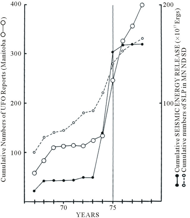
Figure 7. Cumulative numbers of unidentified reports in Manitoba and luminous phenomena reports in three adjacent US States compared to cumulative seismic energy release in the region. Note the increased rate in general luminous phenomena before the 1975 seismic event.
very strong earthquake in Turkey in 1999 [33]. During the weeks that preceded the M9 2011 earthquake in Japan, there was an “epidemic” of reported luminous events across the island. However national media did not report these events because of more pressing political occurrences in North Africa. Only after the tragedy were the phenomena considered important. The Devereux example and the events that occurred in Turkey and Japan emphasize an important principle. If one is not aware of the significance of luminous events and their direct relation to natural processes accompanying tectonic strain that precede earthquakes, the utility of these phenomena to predict earthquakes cannot be realized.
Our research has primarily involved small and medium magnitude earthquakes because of the geophysical nature of the regions we have investigated. There are many examples over the centuries, from China, Japan, Italy, Turkey, and Europe where an “epidemic” of reporting of unusual luminous phenomena preceded major events by months to years. One explanation for the paucity of what should be a conspicuous array of these associations could be the relationship between the magnitude of the imminent seismic event and the distance from the epicentre where strain conditions are optimal for production of luminous phenomena. Rikitake [34] showed a linear relationship between epicentral distance for the observation point for electromagnetic emissions and the energy release of the seismic event. Around magnitudes 7 to 8, the distance exceeded 1000 km.
Stress fields involve large areas of space. Measurements in the changes in tectonic stress fields require an estimated hundreds of thousands of work hours per year. To date one of the most reliable inferences of changes in stress fields before earthquakes may be natural phenomena: luminous displays. Perhaps a Central Registry for these phenomena, whose continuity and financial support would be insured by international law, is now appropriate in order to collect the data with sufficient accuracy to help forecast, if not ultimately predict, earthquakes.
6. Acknowledgements
We thank Professor Blake T. Dotta for technical assistance.
REFERENCES
- M. A. Persinger, G. F. Lafreniere and B. T. Dotta, “Marked Increases in Background Photon Emissions in Sudbury Ontario more than One Week before the Magnitude >8.0 Earthquakes in Japan and Chile,” International Journal of Geosciences, Vol. 3, No. 3, 2012, pp. 627-629. doi:10.4236/ijg.2012.33062
- F. St-Laurent, “The Saguenay, Quebec Earthquake Lights of November 1988-January 1989: A Comparative Study with Reference to the Geoatmospheric Lights Classification Proposed by Montandon in 1948 and a Description Put Forward by Yasui in 1968,” Seismological Research Letters, Vol. 71, No. 2, 2000, pp. 160-174. doi:10.1785/gssrl.71.2.160
- J. Milne, “Earthquakes and Luminous Phenomena,” Nature, Vol. 87, 1911, p. 16. doi:10.1038/087016a0
- I. Galli, “Raccolta e Classificazione di Fenomeni Luminosi Osservati Nei Terremoti,” Bolletino Della Societa Italiana, Vol. 14, No. 6-8, 1910, pp. 221-251.
- T Terada, “On Luminous Phenomena Accompanying Earthquakes,” Bulletin of the Earthquake Institute (Tokyo), Vol. 9, No. 3, 1931, pp. 225-255.
- J. S. Derr, “Luminous Phenomena and Their Relationship to Rock Fracture,” Nature, Vol. 321, 1986, pp. 470-471. doi:10.1038/321470a0
- M. D. Altschuler, L. L. House and E. Hildner, “Is Ball Lightning a Nuclear Phenomena?” Nature, Vol. 228, 1970, pp. 45-46. doi:10.1038/228545a0
- D. Finkelstein and J. R. Powell, “Earthquake Lightning,” Nature, Vol. 228, 1970, pp. 759-760. doi:10.1038/228759a0
- A. I. Grigoryev, N. I. Gershenzon and M. B. Gokhberg, “Parametric Instability of Water Droplets in an Electric Field as a Possible Mechanism for Luminous Phenomena Accompanying Earthquakes,” Physics of the Earth and Planetary Interiors, Vol. 57, No. 1-2, 1989, pp. 139-143. doi:10.1016/0031-9201(89)90223-9
- Q. Chen and A. Nur, “Pore Fluid Pressure Effects in Anisotropic Rocks: Mechanisms of Induced Seismicity and Weak Faults,” Pageoph, Vol. 139, No. 3-4, 1992, pp. 463- 479. doi:10.1007/BF00879947
- Y. H. Ohtsuki and H. Ofuruton, “Plasma Fireballs Formed by Microwave Interference in Air,” Nature, Vol. 350, 1991, pp. 139-141. doi:10.1038/350139a0
- M. A. Persinger, “Transient Geophysical Bases for Ostensible ‘UFO-Related’ Phenomena and Associated Verbal Behavior,” Perceptual and Motor Skills, Vol. 43, No. 1, 1976, pp. 215-221. doi:10.2466/pms.1976.43.1.215
- J. S. Derr and M. A. Persinger, “Luminous Phenomena and Earthquakes in Southern Washington,” Experientia, Vol. 42, No. 9, 1989, pp. 991-999. doi:10.1007/BF01940703
- J. S. Derr and M. A. Persinger, “Luminous Phenomena and Seismic Energy in the Central USA,” Journal of Scientific Exploration, Vol. 4, No. 1, 1990, pp. 55-69.
- M. A. Persinger and G. F. Lafreniere, “Space-time Transients and Unusual Events,” Nelson-Hall, Chicago, 1977.
- P. Devereux, “Earthquake Lights Revelation,” Blandford, London, 1989.
- M. A. Persinger, “Geophysical Variables and Human Behavior: XVIII. Expected Perceptual Characteristics and Local Distributions of Close UFO Reports,” Perceptual and Motor Skills, Vol. 58, No. 3, 1984, pp. 951-959. doi:10.2466/pms.1984.58.3.951
- M. A. Persinger, “Geophysical Variables and Human Behavior: IX. Expected Clinical Consequences of Close Proximity to UFO-Related Luminosities,” Perceptual and Motor Skills, Vol. 56, No. 1, 1983, pp. 259-265. doi:10.2466/pms.1983.56.1.259
- M. A. Persinger, “Geophysical Variables and Behavior: XXI. Geomagnetic Variations as Possible Enhancement Stimuli for UFO Reports Preceding Earthtremors,” Perceptual and Motor Skills, Vol. 60, No. 1, 1985, pp. 37-38. doi:10.2466/pms.1985.60.1.37
- M. A. Persinger and J. S. Derr, “Geophysical Variables and Human Behavior: XXIII. Relations between UFO Reports within the Uinta Basin and Local Seismicity,” Perceptual and Motor Skills, Vol. 60, No. 1, 1985, pp. 143-152. doi:10.2466/pms.1985.60.1.143
- J. S. Derr and M. A. Persinger, “Geophysical Variables and Human Behavior: Annual January Rainfall May Modulate the Incidence of Luminous Phenomena within the San Francisco Basin,” Perceptual and Motor Skills, Vol. 92, 2001, pp. 1180-1190.
- M. A. Persinger and J. S. Derr, “Geophysical Variables and Human Behavior: LXII. Temporal Coupling of UFO Reports and Seismic Energy Release within the Rio Grande Rift System: Discriminative Validity of the Tectonic Strain Theory,” Perceptual and Motor Skills, Vol. 71, No. 2, 1990, pp. 567-572. doi:10.2466/pms.1990.71.2.567
- J. S. Derr and M. A. Persinger, “Geophysical Variables and Human Behavior: LXXVI. Seasonal Hydrological Load and Regional Luminous Phenomena within River Systems: The Mississippi Valley Test,” Perceptual and Motor Skill, Vol. 77, No. 3f, 1993, pp. 163-170. doi:10.2466/pms.1993.77.3f.1163
- J. K. Costain, G. A. Bollinger and J. A. Speer, “Hydroseismicity: A Hypothesis for the Role of Water in the Generation of Intraplate Seismicity,” Seismological Research Letters, Vol. 58, No. 3, 1987, pp. 41-60.
- P. A. Hsieh and J. D. Bredehoeft, “A Reservoir Analysis of the Denver Earthquakes: A Case of Induced Seismicity,” Journal of Geophysical Research, Vol. 86, No. B2, 1981, pp. 903-920. doi:10.1029/JB086iB02p00903
- J. S. Derr and M. A. Persinger, “Quasi-Experimental Evidence of the Tectonic Strain Theory of Luminous Phenomena: The Derby, Colorado Earthquakes,” Perceptual and Motor Skills, Vol. 71, No. 3, 1990, pp. 707-714. doi:10.2466/pms.1990.71.3.707
- M. A. Persinger and J. S. Derr, “Geophysical Variables and Behavior: LXXIV. Man-Made Fluid Injections into the Crust and Reports of Luminous Phenomena Is the Strain Field an Aseismically Propagating Hydrological Pulse?” Perceptual and Motor Skills, Vol. 77, 1993, pp. 1059-1065. doi:10.2466/pms.1993.77.3f.1059
- J. S. Derr and M. A. Persinger, “Geophysical Variables and Behavior: LIV. Zeitoun (Egypt) Apparitions of the Virgin Mary as Tectonic Strain-Induced Luminosities,” Perceptual and Motor Skills, Vol. 68, No. 1, 1989, pp. 123-128. doi:10.2466/pms.1989.68.1.123
- A. El-Sayed, R. Wahlstrom and O. Kulhanek, “Seismic Hazard of Egypt,” Natural Hazards, Vol. 10, No. 3, 1994, pp. 247-259. doi:10.1007/BF00596145
- M. A. Persinger and J. S. Derr, “Geophysical Variables and Behavior: XIX. Strong Temporal Relationships between Inclusive Seismic Measures and Luminous Reports in Washington State,” Perceptual and Motor Skills, Vol. 59, No. 2, 1984, pp. 551-556. doi:10.2466/pms.1984.59.2.551
- M. A. Persinger, “Geophysical Variables and Behavior: XV. Tectonic Strain Luminosities as Predictable but Hidden Events within pre-1947 Central USA,” Perceptual and Motor Skills, Vol. 57, No. 3f, 1983, pp. 1227-1234. doi:10.2466/pms.1983.57.3f.1227
- M. A. Persinger, “Prediction of Historical and Contemporary Luminosity Reports by Seismic Variables within Western Europe,” Experientia, Vol. 40, No. 7, 1984, pp. 676-681. doi:10.1007/BF01949720
- O. Kurtulus, “Faylarin Cevresindeki Tuhaf Gok Olaylari: Deprem Isiklari,” Bilim ve Teknik, Vol. 383, No. 32, 1999, pp. 40-43.
- T. Rikitake, “Nature of Electromagnetic Emission Precursory to an Earthquake,” Journal of Geomagnetism and Geoelectricity, Vol. 49, No. 9, 1997, pp. 1153-1163. doi:10.5636/jgg.49.1153