International Journal of Geosciences
Vol.4 No.1(2013), Article ID:27030,13 pages DOI:10.4236/ijg.2013.41012
On “Voice of Sea” Generation Mechanism
The Academician N. N. Andreev Acoustic Institute, Russian Academy of Sciences, Moscow, Russia
Email: asemen@akin.ru
Received October 30, 2012; revised November 27, 2012; accepted December 26, 2012
Keywords: Infrasound; Sea Surface-Atmosphere Interaction; Whole Gale; Wind Velocity; Oscillation Frequency; Sea Noise; Self-Sustained Oscillations
ABSTRACT
Physical model of self-sustained infrasonic air oscillations related to interaction of fresh gale with choppy sea surface is proposed. It is shown that air infrasonic oscillations are expected inside moving 3D cavities in sea surface generated by gale and detected far from its region. Interaction of wind with moving sea wave crests is shown to be of weaker impact on oscillations in far field. For wind velocity in the range from 10 to 40 m/s deepest cavities acquire resonance frequencies in the range of 3.0 - 0.7 Hz, i.e. frequencies much lower than their quarter wavelength resonance frequencies. In the course of oscillations effective wind velocity applied to cavities can achieve value from 0.4 to 0.6 of wind velocity, while air self-sustained oscillations velocity amplitude can run up in the range from 0.2 to 0.3 of wind velocity. Wind intensification leads to oscillations frequency decrease and oscillation energy losses increase with wind velocity cubed. Cavities natural frequencies are transformed due to air attached mass and volume elasticity additional transformation under wind influence in the range from 1.05 to 1.9 with respect to resonance frequencies at rest. Amplitude of self-sustained oscillation in atmosphere is expected to increase with wind velocity cubed, while cavity air oscillation velocity-linear with wind velocity. Wind velocity threshold of an order of 25 - 30 m/s overcome is necessary to observe effect. Spectral peaks on resonance frequencies in the range 0.7 - 2.5 Hz are expected in effect observation. Infrasonic signals observable far from whole gale in atmosphere, sea water thickness and earth crust on self-sustained oscillation frequency and its harmonics frequencies beginning from third harmonic 2.1 - 7.5 Hz are regarded as phenomenon signs.
1. Introduction
Problem of wind flow interaction with troubled ocean surface attracts scientist attention for a long time [1-33]. As early as in XVIII century observations allow developing scales of sea roughness and wind which are used with minor corrections until now. Most important experiment and theory results were obtained in ХХ century. It is well known that propagation of slow enough wind waves over ocean surface can not lead to atmosphere infrasonic sound wave radiation [2,11-13]. Troubled surface interaction with wind is bound up with high-speed atmosphere turbulent stresses spectral components propagating with velocity exceeding atmosphere sound velocity [14]. Evidently, such properties could be expected from not bearing wind turbulence basic power turbulent fluctuation spectrum “tails” only. However even those statistical in nature continuously depending on wind velocity processes can not explain phenomenon of sudden appearance of powerful infrasonic signals observed far from heavy gale region in conditions where wind velocity overcome a kind of threshold-so called “voice of sea”. Seemingly, first time “voice of sea” was detected experimentally by academician V. V. Shuleikin [1,3] in the last century 30-th years. In accordance to his observations, “voice of sea” is narrow band infrasonic signal detected on frequencies below 6 - 10 Hz. But there are valid enough doubts in phenomenon frequency evaluation on the basis of balloon filled with hydrogen resonance frequencies. For instance, lowest axisymmetric balloon oscillation frequency 2 - 3 Hz was inexplicably excluded from evaluation. Various considerations on uncommon effects related to “voice of sea” were proposed, say, on infrasonic signals negative influence on man’s mentality. Influence of “voice of sea” infrasound was even proposed as an explanation of ships and yachts crew traceless losses. While ships itself were found in good enough state. Apart from V. V. Shuleikin phenomenon explanation attempts were undertaken by several eminent physicists including academicians N. N. Andreev [2] and B. P. Konstantinov [4]. Explanation attempts are undertaken until now. For instance in [24] noise amplification capability in sound waves reflection from troubled sea surface based on known Miles model [16] was demonstrated. In the presence of supposed infrasound sources this effect is proposed as possible “voice of sea” mechanism. However, sources origin or, in other words, infrasonic phenomenon generation mechanism remains not understood, while authors mentioned proposed qualitative considerations. In particular, N. N. Andreev [2] proposed a hypothesis that probably “voice of sea” is sequent of air vortex separation in wind interaction with ocean wave crests. Expected phenomenon frequency estimates were even proposed, but few important questions remain unanswered until now:
• What is the source of “voice of sea”?
• What is “voice of sea” spectrum?
• How spectrum depends on wind velocity?
• How effect intensity depends on wind velocity?
• At what velocity is effect revealed?
From our point to answer them it is necessary to look on results of acoustics and subsonic gas dynamics studies more fixedly.
It is known that external potential flow of ideal fluid over 2D obstacles on the plane is examined in classical hydrodynamics [5]. For single obstacles of simplest shape classical method is based on description of flow by complex potential in coaxial coordinates. Typical examples of such obstacles are shown on Figure 1. 2D obstacles—lug and cavity situated between points А and В, equidistant from obstacle center in point O on x axis at distance b.
Not going into details of solutions we remind simplest obstacles basic results. Smooth lugs are characterized by velocity finite value in all points of flow (including points А and В), while for simplest semi-cylinder lug velocity at its vertex is equal to 2U, where U—incident
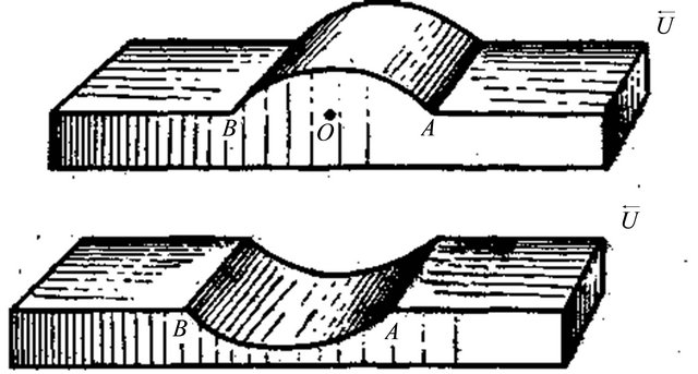
Figure 1. Ideal fluid external flows over 2D obstacles (lug and cavity) calculation outline [5].
flow velocity at infinity. In 3D case for semi-sphere lug the flow is potential, while vertex velocity is equal to 3U/2. For sharp lug vertex velocity is infinite. For cavities velocity turns to infinity at point А and В, while at the bottom of simplest semi-cylinder cavity velocity is equal to 2U/9. In 3D case for semi-sphere cavity bottom velocity is also finite, but flow inside cavity cannot be described by velocity potential. It is vortex and close qualitatively to flow inside Hill vortex [5].
In media of finite viscosity at large Reynolds numbers perceptible difference in these obstacle impact on ambient flow is observed [6,7,9]. In fact streamlined obstacle flow pattern is notable from ideal fluid by boundary layer presence only. At large Reynolds numbers its thickness is negligible and, while it increase with distance from obstacle, but it is easy to show [9], that its transverse scale  ratio to characteristic longitudinal scale
 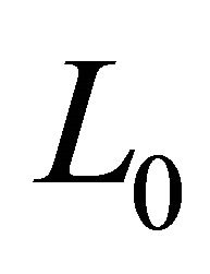 is expressed
 .
.
For instance at flow velocity 10 m/s beyond obstacle (lug) leading edge boundary layer thickness at distance 100 m makes not more than 1.5 cm. This flow property allows ignoring boundary layer in low frequency instability study of cavities situated between lugs avoiding noticeable errors. At the same time this thin layer possesses internal instability defining its growth and responsible for wind power transfer to ocean surface. In the frame of reference moving with waves the way of relative horizontal velocity change in “matched” layer evidences its transition through zero and positive velocity values achievement above layer. Besides, even in 2D phase-averaged turbulent flow pattern near matched layer existence of closed flow lines related to vorticity initiation in cavity inflow is observed [12]. Corresponding flow lines in the frame bounded to wave are shown on Figure 2.
This purely kinematic result obtained for realistic fluid flow corresponds to ideal flow over cavity near points А and В on Figure 1, where infinite velocity values were noted [5].
Cavity around flow is well studied experimentally [7].
Figure 2. Phase-averaged 2D picture expected in the frame moving with waves in cavity inflow near matched layer in turbulent wind flow over ocean surface [12]. Closed lines centers correspond to matched layer.
As we have already mentioned, vortices and discontinuity surfaces are generated on sharp cavity edges. If cavity width is small and edges are smooth enough then flow over cavity remains almost unchanged. However with cavity width increase (or for sharp edge cavities) its reaction changes, flow boundary dynamics, instability and boundary oscillations come into force. The flow tends to leak into cavity providing conditions for self-sustained oscillations generation. If flow meets wave crest, say wind catch up wave crest on sea surface then at first moment flow over it is observed, while due to theory prediction velocity value there is very large, in theory—up to infinity. However, observations evidence that such flow regime leads to rapid vortex formation and edge velocity decreases. To explain this phenomenon in hydrodynamics the principle [7] is used in accordance to which realistic flow tends to avoid infinite flow velocity transforming flow near these points to discontinuity surfaces. That is why conditions of vortices and discontinuity surfaces generation are provided near wave crests. While vortices and discontinuity surfaces as a whole are growing together even from small enough initial disturbance [7].
Troubled sea surface far from shore itself is not capable to radiate low frequency homogeneous sound waves propagating in atmosphere [9,11-13]. As it is already specified, radiation requires sea surface disturbance (say, wind disturbance) Fourier integral decomposition component wavelength exceeding air sound wavelength. This condition possible exception is related to marginal effects only, observed mainly in wave interaction with shore line [4]. For instance, on sea roughness spectrum maximum (near 0.1 Hz) surface wavelength is close to 150 m, while corresponding air sound wavelength—close to 3000 m, which blocks homogeneous wave radiation. Radiation conditions on higher frequencies are even more unfavorable [11].
In the same time besides stochastic turbulent tangential stresses on ocean surface situated close to matched layer mentioned above there are localized low frequency sound sources related to wave crests and cavities on troubled sea surface generating self-sustained oscillations under wind influence.
2. Oscillations Environment
Necessary condition of self-sustained oscillations is wind velocity exceeding largest wave crests velocity. For sea roughness spectrum is continuous while ocean waves has rather trochoidal than sinusoidal shape, surface wave group velocity should be used as main absolute physical wave motion characteristics. In other words, largest wave crest or wave cavity motion is a source of whole spectrum of sinusoidal wave’s motion. According to theory 2D sinusoidal surface waves group and phase velocities relation depends on wavelength and sea depth relationship and changes in the range from 0.5 to 1 for depth change from infinity to zero. Group velocity differs considerably from phase velocities of isolated wave crests and cavities. However, from the point of isolated cavity oscillations excitation main role belongs to positive difference between wind and definite cavity phase velocity. For instance, in intensive roughness surface oscillation spectrum maximum is close to . In 2D wave pattern it corresponds to crest phase velocity
  (g—gravity acceleration) independent of wave amplitude. That is why at wind velocity lower than
  self-excitation is impossible. As we have already noted, in theory group velocity is two times lower. In accordance to Newman and Pierson [12] group velocity depends on wind velocity as well
  , so that difference of wind and group velocity
  equal to
  act on large cavities of not sinusoidal shape. Such estimates are fair however for wind roughness starting zones only and in swell conditions only. In gale initiation realistic wind roughness far from the shore is 3D in fact. According to contemporary theory wind power transfer to waves is reduced to 2D roughness transition to 3D. In swell development transition of 3D roughness back to 2D is observed [3].
Thus, widely spread notation on rough sea surface 2D form [24], reminding washboard is inaccurate. Sea surface photo even at low enough wind velocity evidences that sea surface is not 2D [3]. It is rather 3D and reminds chessboard. Sea surface shape is schematically shown on Figure 3.

Figure 3. Schematic structure of troubled sea surface comprising set of lugs and cavities of various scales with respect to axis x and y. Wind of velocity U is directed along x axis [3].
Its squares are made of finite in horizontal dimensions (length and width) crests and quasi rectangular cavities situated between them. Geometrical dimensions and depth of cavities increase with wind intensification. They have form of surface recesses—open soap cases with rough edges where depth h is several time less than horizontal dimensionsв of rectangle cell . Here d—cell dimension along wind direction, across wave crest, while b—cell dimension along wave crest. In 2D roughness pattern at swell conditions wave phase velocity can exceed wind velocity and it leads to wave power losses. However in gale development to 3D pattern it is impossible. According to [3] longest 2D waves phase velocity
  ratio to wind velocity
  beyond developed swell limits is not more than
 . Maximum wave length
  in SI system of units comprises around
 , wave period
  comprises
 .
.
Cavity slope  is up to
[3]. As to cavities geometrical dimensions relationship, it follows from wind waves spectrum study that space correlation radius  of sea surface elevations with respect to crest normal is limited and small enough. In an order of magnitude it comprises less than tenth part of wave length
 .
.
Correlation radius along wave crests  comprises not more than two tenth parts of wavelength
 .
.
Their ratio is equal approximately to  [15]. In further problem solution we take ratio of
  on that basis. Phase velocity
  of 3D waves turns out to depend on this ratio value [3]. Phase velocities relationship of 3D
  and 2D
  acquires the form
 i.e.
i.e. , while in wind direction
 .
.
Taking into account velocity value , the value
  equals to
 . Thus, actual phase velocities difference
 , influencing on isolated cavity is 0.59U. It is comparable to wind and group velocities difference of 2D waves 0.39U. Choosing velocity difference in these limits we take into account realistic gale wave spectrum inharmoniousness. Large cavities depth (from crest to bottom) has dispersion from 2 to 30 meters (in the mean around 10 - 15 m) for wind velocity
  from 10 to 40 m/s. Horizontal cavity dimensions are in an order more.
3. Resonance Frequencies
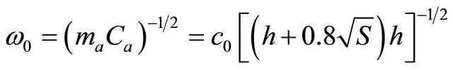
This environment defines cavities low frequency (infrasonic) characteristic resonance spectra. Apparently, corresponding oscillation frequencies are grouped around resonance frequency of average depth cavity. For all such cavities are pyramidal in volume shape with of almost rectangular section and upper cover in the form of massive enough cavity piston of surface density
 then positive resonator conductance
  equal to
  [11]. Neglecting losses resonance frequencies equation takes the form
 . (1)
. (1)
Particular solution of it is simplified for . We note that
  ratio accounting to cavity rectangle side relationship
  takes the form
 .
.
Expanding left side of (1) in series at , we obtain equation
 . (2)
. (2)
Its solution < say, at  leads to sound wave length value
 , i.e. ultra low frequency oscillations are possible in cavity volume where only small fraction of wavelength corresponds to cavity depth
 . In low frequency oscillation of that type cavity medium is working just like spring. At parameter values chosen
  3 - 15 m cavity resonance frequency is in the range from 0.7 to 3.4 Hz in the absence of wind. Experiments data adduced in [21-23], evidence air adjoined mass value taking part in resonator oscillations dependence on flow velocity. It turns out, that flow velocity increase leads to adjoined mass decrease down to half of it at flow velocity comparable to resonator oscillation velocity. That is why in resonator frequency evaluation we take into account adjoined mass behavior considering
  equal to
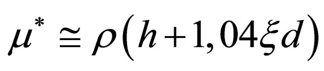 , where mass losses factor
  changes from 1 to 0.5 due to relative velocity
  change from zero to
 , where a—resonator oscillation amplitude. For
 , cavity resonance frequency is increasing approximately from 1 to 1.4 times with respect to cavity frequency in the absence of wind. In wind increase up to value
 , factor
  fall to zero and become negative at
 , corresponding to cavity opening impedance nature change from “mass” to “elastic” type [31]. If resonator opening will be examined as obstacle for sound wave and take oscillation amplitude
  as obstacle characteristic dimension, while ratio
  as modified obstacle Stroukhal number
 , then taking into account experimental study [21] we shall see that obstacle behaves as mass in the range
 , and it behaves as elasticity at
 . In Stroukhal number range from 0.15 to 0.25 cavity upper section resistance is negative and its self-excitation is possible. This result disprove partly hypothesis of paper [2], where vortexes separation from semi-cylinder wave crests are supposed to be a source of “voice of sea” at Stroukhal number value
 , ignoring role of cavities. However, as we shall see below, this source model is to be rejected in relation to generated sound field directivity far from the sources as well.
Let us suppose that cavity upper cover reactive conductance is of an order of medium conductance . Then, considering
  and comparing cavity upper cover conductance real
  and imaginary
 part values of total conductance
  and then accounting for conductance related to sound radiation in atmosphere half space
 , we obtain estimate
 . With correction to oscillating mass
 , i.e. at
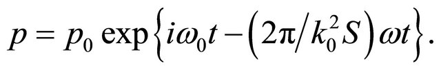
 evaluated product is comparable to unity in an order of magnitude. With aid of known solution for pressure field in cavity at
 [11], in first approximation in
  (
( or taking into account adjoined mass correction
 ) we obtain expression for decaying pressure field in cavity
 (3)
(3)
It is evident, that oscillation frequency changes (in the case of mass cavity cover —increases) due to small enough resistance in second order. In first order approximation frequency is unchanged [11]. For small enough frequency
  cavity resonance oscillation pressure field (3) takes the form
 (4)
(4)
On cavity upper cover at ,
,
Corresponding force , acting on flow in upper cavity section has the form
 , where
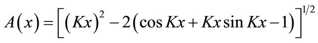
In other words, if outer flow would be absent, the decaying oscillation will be observed in cavity with quality factor of an order of unity. It is known that at  attenuation
  leads to oscillation amplitude restriction during cavity excitation under influence of force
 , while maximum amplitude is proportional to applied force. Outer flow is a factor supporting oscillations in cavity, i.e. compensating oscillation fast decay. Natural resonance oscillations have low enough quality factor
 . Taking into account wind influence on adjoined mass range of resonance frequency change turns out to be from 0.7 to 4.8 Hz. Cavity depth increase is equivalent to oscillatory circuit capacity, it leads to frequency decrease and vice versa decrease of cavity depth leads to frequency increase. Cavity upper section horizontal dimensions increase leads to frequency decrease, while horizontal dimensions decrease—to frequency increase.
One more factor influencing frequency of cavity resonance oscillation is resonator elasticity parameter (compressibility of cavity volume) depending on tension force value and oscillations amplitude. In fact, taking resonator pyramidal volume , upper cavity section displacement
 , atmosphere pressure
 , specific heats ratio
 , while pressure and volume disturbances
  and
and 
 respectively and expanding adiabatic law expression for resonator volume in Taylor series
 , (5)
, (5)
We obtain at  for pressure fluctuations in resonator ordinary expression
 . (6)
. (6)
Second term of Expansion (6) generally has no relation to volume compressibility—it is simply square correction to pressure amplitude in cavity on resonance frequency—“second harmonics”. Actual correction value (second term factor) is to be specifically calculated for each resonator oscillation mode. Evaluation of this factor for resonator is known. For instance, in resonator with one rigid and one soft covers second harmonics of basic resonance frequency is not observed for there are no even harmonics in oscillation spectrum [11]. That is why second expansion term could be neglected and then for resonator nonlinear compressibility term we have ordinary expression
 .
.
Here —oscillation amplitude value at which nonlinear terms contribution in system elasticity is comparable with linear term contribution. As a result we have
 , while
 .
.
Oscillation frequency  of such system is equal [13]
 . (7)
. (7)
where we have denoted—system elasticity tension
 ,
,  ,
,
 ,
,
 —driving force. We note, that condition
 is fair when
 , which is uncharacteristic for the case under analysis. At
  second summand in expression for
  turn out to be negative and expression takes the form
 .
.
Thus, independent of force nature stretching system elasticity oscillation frequency increases. The value 
 is defined by pressure force applied to cavity upper section and is independent of resonator volume. If difference between static pressures in atmosphere (accounting for wind of velocity
 ) and in cavity (air at rest) is examined as stretching force, then ratio value
  could be evaluated by expression
 where
where —resonator drug factor. Ratio
 changes from
  to
to  in our case with wind velocity U changing from 10 to 40 m/s, while
  changes in the range
 . Besides due to influence of adjoined mass correction in Stroukhal number range Sh > 0.1, as we have seen above, frequency changes in 1 - 1.4 times with respect to value in the absence of wind. As a whole, actual cavity resonance frequency changes with wind velocity in the range from 1 to 1.9 of value
  in the absence of wind, i.e. from 0.7 to 6.5 Hz in absolute value. Upper frequency limit corresponds to fresh gale
 , while lower—to heavy gale
 . It should be noted, that with wind increase self-sustained oscillations may cease due to losses increase.
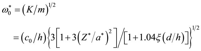
Taking into account cavity depth and horizontal dimension dependence on surface wavelength it could be shown for 2D waves that resonance frequencies of deepest cavities are close in an order of magnitude. For given wind velocity they are proportional to ratio of sound velocity in atmosphere  to surface wavelength
 . (8)
. (8)
Due to surface wavelength proportionality to squared wind velocity, cavity resonance frequency decreases with wind velocity squared. Frequency values are in the range from 5 - 7 Hz at  until 1 - 0.5 Hz at
 . These estimates are close to oscillation frequency range, evaluated above on the basis of cavity lumped system parameters in the wind. Self-excitation of largest cavities is possible in the case of wind velocity excess wave velocity, i.e. at
 . Wind direction however not always coincides with normal to wind crests [14]. This fact was partly taken into account in evaluation of velocity difference
  in the range
 , influencing on cavity in the frame of 3D surface wave model. In 2D model the value of
  is also positive, with exception probably of gale swell regime and comprises
 .
.
Let us suppose that wind is directed along x axis, y axis is normal to wind velocity in horizontal plane, while z axis is directed upwards and normal to horizontal plane. We adduce one more argument for sound sources selection defining possible self-sustained oscillation contribution in far sound field. Let us take into account that longitudinal mode of cavity oscillations comprises monopole source “underlined” by sea surface in atmosphere half-space sound radiation. Then source related to flow self-sustained oscillation due to vortex separation from wave crests comprises vertical dipole sound source with minimum directionality in horizontal direction weakened by sea surface. In fact, latter source far field is reduced to quadruple field. In addition to hydrodynamics argument proposed above, this argument substantiates source model choice from the point of acoustics in favor of cavity longitudinal oscillations. It is also additional argument in possible “voice of sea” mechanism discussion [2].
4. Oscillation Losses
Now it is time to analyze basic losses sources related to sea surface cavity inner volume oscillations. In their low frequency oscillations following factors are of importance—it is viscose attenuation of sound in cavity volume and on cavity walls, radiation of sound in atmosphere and then (with amplitude increase) it is nonlinear (aerodynamics) resistance related to influence of stationary outer flow. Part of power at high oscillation intensity could be probably transferred to second harmonics power. But for the case of air oscillations in cavity with rigid bottom and opposite open end even harmonics are not allowed.
Viscose forces work transferring acoustic oscillations power to heat calculated per unit volume in medium is proportional to , while power spent in viscose boundary layer to
 .
.
Taking into account pyramidal cavity shape mentioned volumes are equal to  and
and  respectively. Lost power ratio acquires the form
 . It is easy to see that for low frequency case losses are defined by absorption in boundary layer [11]. In the same time they are negligible with respect to radiation losses.
Cavity horizontal dimension , as a rule, is larger than its depth
 . As we have seen, wave length of cavity super infrasonic resonance
  and thus value
 defining monopole source reactive and active power ratio evidence that they are comparable. At given radiation power value reactive power is an indicator of source minimum operability. Thus for insufficient inflow power (volume velocity) entering cavity spent for self-sustained oscillations support, necessary condition of their existence could be violated and oscillations itself could be stopped. However, redundant inflow, say, related to wind increase leads to oscillation stop due to nonlinear hydraulic losses increase.
For hydraulic nonlinear losses evaluation we shall proceed from pressure losses factor  observed for cavity (opening) oscillating flow in the presence of outer flow (wind) over opening upper section [34]. At air oscillation amplitude
  of frequency
  oscillation velocity comprises
 . Then hydraulic pressure losses equivalent to additional force applied to resonator comprise
 ,
,
 .
.
Hydraulic losses factor value  increases with ratio of
  to
to  increase. Change of
  with ratio
  for the case of rectangular opening with dimensions relationship
  is shown schematically on Figure 4.
Nonlinear character of resistance value dependence on  in the range from 0 to 1 is important for self-sustained oscillationв excitation (Figure 4). For ratio increase above 1 losses increase suppress oscillations. For ratio value
  losses factor
  achieve 7 ([34], p. 178). Ratio
  value depends on frequency and power of self-sustained oscillation. Values of factor
  are summarized in Table 1.
Curve on Figure 4 could be expressed explicit in the form
 .
.

Figure 4. Dependence of pressure losses factor ζ on ratio  in outer flow (wind) percolation over opening in rigid wall with velocity U0 [29] and oscillating flow with velocity aω through opening.
Table 1. Opening resistance in flow.

Here ,
, —normalizing factor and its value
 , while
 . Thus expression for additional force
  comprises three summands
 . (9)
. (9)
At  (9) is reduced to first term equal to zero for U0 = 0. It corresponds partly to additional static tension of cavity elasticity. Total tension force
  value comprises
 . At
. At  second and third terms of
  in (9) come into force. Second term corresponds to negative acoustic resistance for sign-changing flows in resonator. This term is close in sense to resistance observed in experiments [21], but air compressibility is ignored. And, at last, at
 , second and third terms are principal. That part of active resistance (9) is positive at
  and negative at
 , it corresponds qualitatively to opening impedance measurement in flow data [21]. Last term of (9) provides oscillation suppression at definite value of
 , with increase of
 .
.
Nonlinear losses influence on excitation of self-sustained oscillations seems to be evident. But from the moment when the question of nonlinear losses fine structure influence on Helmholtz resonator behavior in intensive acoustic field was stated in [19] there are practically no study that take this losses type into account. Nevertheless second term influence in expression for  on acoustic resistance of oscillation systems (say, pendulum) in flow is noted in [13].
5. Wind Dependent Impedance
In finite opening of area  streamlined by flow in its plane there are few specific features to be observed. They are expected for instance in sound wave of wave vector
  reflection from opening. For instance, even for bottomless opening at
on frequency corresponding to opening equality to negative resistance related to second term of (9), for  self-excitation is possible. In spite of not taking into account of such effect in [21,22] their experiment data indirectly evidence its influence. For instance, in accordance to their data, at upper section dimension
  m in wind velocity range from 10 to 40 m/s self-excitation frequency range comprises several tenth of Hz, i.e. almost in an order higher than predicted for “voice of sea” frequencies. Probably it may evidence possibility of reflection of sound wave with reflection factor exceeding unity. In [24] such mechanism was supposed to be responsible for “voice of sea” explanation in 2D wave model. Typical experiment diagram of imaginary
  and real
  parts of circular opening dimensionless impedance reciprocal change with
  is shown on Figure 5 [21].
Opening impedance spiral diagram form is characteristic for impedance diagrams of elements providing sound waves attenuation. If we introduce notion , in Equation (1), it takes the form of logarithmic spiral equation in complex plain
 .
.
Its form and relation with element attenuation and reflection characteristics is discussed in acoustics courses [11]. Same characteristic types are related to sea surface cavity (resonator) opening upper section in flow. Element attenuation characteristics are defined by spiral “twirl”. Spiral characteristic angle defined by ratio of imaginary and real impedance parts serves as attenuation measure. In the simplest case it is independent on frequency and constant. Characteristic angle on spiral of Figure 5 is a value dependent on frequency. In other words, Figure 5 shows impedance diagram with strong enough sound attenuation properties (slow spiral “twirl”), where imaginary and real parts ratio aims at zero for high frequency limit. This conclusion is supported by spiral close to ring form near its root. In the range of parameter val-

Figure 5. Typical experiment diagram of imaginary  and real
  parts of circular opening dimensionless impedance reciprocal change with
  in sound field under outer flow influence. Imaginary
  and real
  impedance parts are depicted on diagram ordinate and abscissa axis respectively. Ratio of flow and sound wave oscillation velocities near opening
  serves as dependence parameter [21]. Values of parameter
  are shown by figures on diagram spiral. Measured impedance values are shown by
  symbols, while interpolated values by
  symbols.
ues  its shape is related directly to hydraulic resistance influence. In that velocity range, real impedance part
  changes sign and achieves negative values corresponding qualitatively to minimum of hydraulic resistance on Figure 4. In the same tine impedance imaginary part in the range of
  from 0 to 1.0 is positive (impedance mass type) and changes from 1 to 0.5. Further on (with increase of
  or decrease of
 ) it aims to constant negative value—providing conditions of purely elastic impedance. Even
  increase until value of 1.25 at
  is registered. It is related probably with the role of compressibility in flow structure reconstruction over opening. With further parameter increase however style of impedance imaginary part behavior changes gradually achieving zero value at
 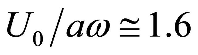 and transforming from mass to elastic impedance type. This transformation corresponds to decrease of oscillations amplitude or frequency. In the same time increase of impedance real part
  with increase of
  corresponds qualitatively (neglecting compressibility) to data of Table 1 and Figure 4. Flow resistance at large values of
  increases with flow velocity squared in accordance to Figure 4 data and not linear in velocity as it is alleged in [21]. Besides, experiment data of Figure 5, obtained without cavity resonance properties accounting evidence transition of impedance real part to small positive values of an order of 0.1 (oscillation attenuation) at Stroukhal number of an order of 0.27 - 0.23 calculated on the basis of oscillation amplitude. It corresponds to values of
  in the range from 0.6 to 0.75. Oscillation amplitude decrease corresponds to negative resistance range, i.e. to maintenance of self-sustained oscillations, while amplitude increase is provided by additional flow boundary oscillation power. For average oscillation amplitude choice in the range of
  (spiral left boundary on Figure 5,
  ) impedance real part with amplitude increase will correspond to negative resistance range—i.e. to self-sustained oscillations maintenance. For amplitude decrease upper cavity section properties are still in “mass” type impedance limits corresponding to cavity oscillation on lowest frequency (1). Further increase of
  parameter (decrease of oscillation amplitude) is impossible for opening in the plain, for at
  cavity upper section acquires impedance “elastic” type value not complying with oscillation character described by Equation (1). However, our estimates are presumably of qualitative type evidencing the reason of preliminary amplitude choice at
  for further evaluations. In the same time these estimates allow to specify the range where self-excitation of cavity with aid of outer flow is possible. But for all that we see that smooth oscillation increase with wind velocity is impossible. On the basis of Figure 5 data analysis, self-excitation effect is expected to origin as sudden jump for flow velocity achieving the value higher than some definite velocity. Due to (8) and (9) we obtain parameters to be used further in oscillations power balance estimates—choosing ratio
  and taking
  we obtain amplitude
 oscillation velocity
 , resonance frequency
  and hydraulic resistance force
  all measured in International units system As before it was supposed, that wavelength
 , while largest cavities depth is
 . Cavities upper section minor horizontal dimension for all that is
 , while upper section area
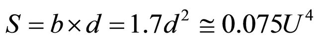 .
.
6. Oscillation Power Balance
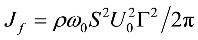
Three components are to be evaluated in oscillations power balance—power of radiated sound field , leaving source, power spent on field reactive component support
  and losses power
 , related to hydraulic flow resistance. In self-sustained oscillation these components are to be compensated by inflow oscillation power
 , of outer flow entering cavity. As to
 , for semi-space radiation it takes the form
 (10)
(10)
If dependence of on
on  is taken into account then dependence of
  on
on  is of an order
 . Preliminary quantitative estimates evidence sound pressure level expected in strong gale region is up to 145 - 150 dB. Reactive power
 , which the source should provide is defined as
 , where
—total reactive energy in semi-space of incompressible fluid equal to adjoined mass moving with velocity  in upper source section energy [11]. Then we have
 (11)
(11)
Hydraulic losses power is defined as force
  (9) work in unit time
  and takes the form
 (12)
(12)
And, at last, power , introduced by outer oscillating flow inside source (cavity) is defined by product
 where
where —outer flow fraction entering cavity, while
  ratio of flow deflection amplitude
 on upper section leeward side to section width. It is possible to calculate this parameter strictly in condition of self-excitation prediction [4]. At
  it leads to estimate
 . Here
  is hydrodynamic wave number of disturbances on outer flow surface. Examples of calculations related to various jet flows are given in [25]. Power
 takes the form
 (13)
(13)
Making up power balance  and using relationship for summands obtained above and for upper section area
  we receive expression for
  in the form
 (14)
(14)
We note, that first and second (14) terms corresponding to  and
and , are comparable. With aid of obvious requirement
  we obtain wind velocity lower limit estimate necessary for phenomena observation
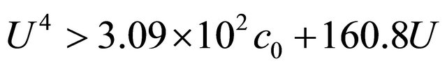 . (15)
It is expected at velocity  only. However, flow deflection
 preliminary estimates evidence that value of
 , should be not more than several tenth in radian or 10 - 15 grade. It corresponds to minimum wind velocity estimate not less than 25 - 30 m/s, which in its turn lead to cavity resonance frequency range 0.4 - 0.8 Hz or taking into account corrections influencing cavity adjoined mass and elasticity under influence of wind— frequency spectral maximum 0.7 - 1.6 Hz. As a whole, accounting for low enough cavity oscillations merit factor and cavities dimension usual spread self-sustained oscillations “voice of sea” spectra are to be observed in the frequency range 0.7 - 2.5 Hz.
7. Self-Excitation Conditions
Adequate calculation of oscillations self-excitation conditions is possible on the basis of two factors influence. First of all, it is phenomenon of purely dynamic (forced) action of sound disturbances (standing waves in cavity) on flow particles moving in outer flow with amplification factor  [4]. And second, it is phenomenon of flow boundary disturbances amplification (resonance oscillations of boundary) due to hydrodynamic instability observed even in the absence of sound with amplification factor
  [26-28]. On low frequencies factor
  is proportional in magnitude to dimensionless flow boundaries onset amplitude [4]
 Which at
  tend to
 .
.
In accordance to theoretical and experimental data
[26-28], flow boundary behind wave crest tangential discontinuity disturbances increase exponentially with distance from crest. In [26] disturbances space growth increment  is calculated for boundary layer profile of the form
 .
.
Increment values are related to momentum boundary layer thickness
 .
.
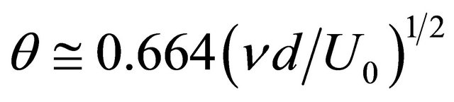
This parameter is almost equal to ordinary boundary layer thickness [9], adduced in paper beginning. Layer thickness on lee cavity edge is
  M. In the range of Stroukhal number
disturbance amplitude growth is characterized by amplification factor
 .
.
Experimental measurements data for space growth increments of disturbances on flow boundary at flow velocity 8 m/s for axisymmetric and plane flow are shown on Figure 6.
It is obvious that best degree of agreement is noted in low frequency part of Stroukhal number range—part I for Stroukhal number values  while this range corresponds entirely with expected conditions of

Figure 6. Dependence of boundary layer disturbances spatial growth increment , calculated with respect to momentum boundary layer thickness
  for flow profile
  in Stroukhal number range
  (solid curve). Experimental measurements data for space growth increments of disturbances on flow boundary at flow velocity 8 m/s are depicted for axisymmetric flow by ○ symbol, while for plane flow by □ symbol. Vertical dotted lines divide regions of various
  values (parts I, II, III), where various agreement degrees of theoretical predictions with experiment data are observed [26].
“voice of sea” development at . For wind velocity
  change from 20 to 40 m/s Stroukhal number changes from 0.013 to 0.006, while disturbances amplification factor
  in the frame of such estimates may achieve values from 1000 to 600 respectively. Total amplification factor
  is to be evaluated as value in varying limits
 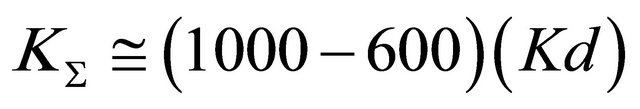 t for stationary flows. For the case of non-stationary flows the value of
  will decrease and previous estimate is to be examined as upper estimate for “voice of sea” observation conditions. It allows defining conditions of self-excitation and range of possible parameter
  values taken as unity on the basis of experiments [21] more exactly. To realize it we shall analyze equation of cavity oscillations as lumped mechanical system.
8. Oscillation Equation
Let us suppose that resonator (cavity) is oscillating as electroacoustic lump system obeying linear equation for displacement of medium particles in cavity volume :
:
 . (16)
Natural (free) oscillations resonance frequency , is expressed in the form:
 . (17)
While oscillations decay factor  is expressed as
 .
.
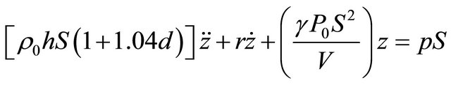
Taking into account lump parameters dependence on wind velocity Equation (16) acquires the form:
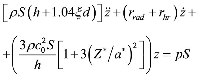 . (18)
Here  cavity radiation resistance,
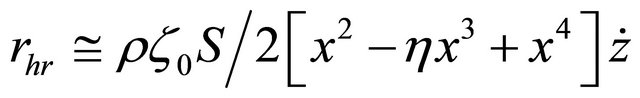
expression for nonlinear hydraulic opening resistance corresponding to expression for hydraulic force  (9). First term of (9) is retained as constant tension force applied to cavity and taken into account in expressions for
  and
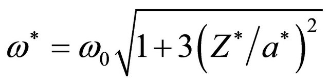
and . Updated expression for resonance frequency
  takes the form:
 .(19)
.(19)
In contrast to ordinary expression (17), recent expression depends on wind velocity absolute value  through cavity medium elasticity (fraction numerator second term under radical) and velocities difference
 , influencing on cavity (fraction denominator second term under radical through mass losses factor
 ).
).
Equation right hand side (driving force) is defined by outer flow reaction and may be written in the form
 . (20)
where —cavity oscillation phase,
 —air jet deflection phase on cavity lee end,
 —phase of maximum jet deflection inside cavity in relation to maximum displacement
  of cavity particles. Position of flow in relation to cavity edge defines phase
  changes in limits from 0 to
  [4]. Phase
  value is equal [4]
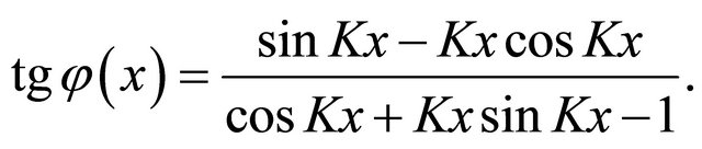
At large  value on cavity lee side for
  expression takes the form
 .
.
Flow influence force in its boundary small oscillation is proportional to boundary oscillation amplitude on cavity lee side or to volume velocity introduced by flow in resonator
 .
.
Expression (20) takes the form
 . (21)
After substitution of all parameters in Equation (18) and comparison of equation left and right sides we obtain condition for stationary self-sustained oscillation definition. It is based on expression for hydraulic resistance (9) nonlinearity and on Equation (18) second term total factor at  equality to zero (lossless oscillations). It allows evaluating self-excitation phase condition as well [25]. But present study is restricted to “voice of sea” generation possibility demonstration only and that is why phase condition is not considered. After substitution in (19) we obtain equation for acoustic velocity magnitude
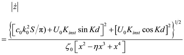 (22)
(22)
It is taken into account that . With aid of condition
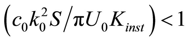 meaning that
 , after few simplifications we obtain nonlinear relationship for parameter
  evaluation
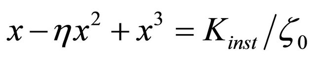 . (23)
It is time to remind that , while
  (c.f. Table 1).
9. Discussion
First term under root in numerator of (22) corresponds to equality of radiation resistance together with hydraulic resistance linear summand real part and injected in cavity flow resistance—real part of nonlinear hydraulic flow resistance. Second term under root corresponds to equality of flow resistance and nonlinear hydraulic resistance imaginary parts. Calculations show that minimum selfexcitation amplification factor value  is of an order of 20
 , the value much less than maximum value predicted in Section 7, parameter
 is of an order of 1.8, which is comparable in principle to value
 , used for evaluation with aid of [21] in Section 6. This estimate confirms possibility of oscillation self-excitation. Amplification factor
  growth leads to parameter
  increase and consequently to stationary oscillation amplitude decrease. The limit here is provided by change in upper cavity section impedance type from “mass” to ”elastic” say, as for opening in the plane at
  [21]. Formally decrease of parameter
 is possible, but in fact condition
  will be violated. Thus realistic value of
 is to be chosen as
 . At
. At  inequality (15) takes the form
  Limiting (threshold) velocity beyond which self-excitation is expected at
 , turns out to be equal to
 . Oscillation amplitude decreases with respect to predicted above at
  almost in 2 times. In other words, sound pressure level in heavy gale zone comprises up to 140 - 150 dB in these conditions.
Powerful infrasonic field generated in atmosphere over sea surface penetrate in sea layer due to cavity walls oscillations and through sea bottom penetrate to earth crust. Infrasonic noise far from whole gale in atmosphere, sea water thickness and earth crust with peaks on natural frequency 0.7 - 2.5 Hz and their harmonics frequencies beginning from third harmonic 2.1 - 7.5 Hz (c.f. Section 3) is expected in phenomenon observations. Naturally the distance from the gale center plays no substantial role in phenomenon observation. For instance if we evaluate the gale zone dimension as 500 km, at distance 5000 km sound pressure level mean square value changes on not more than 10 - 20 dB only, hardly preventing their observation. Almost 80 years passed from “voice of sea” first observations [1-3]. However observations of infrasonic signals with characteristics close to predicted for “voice of sea” in ocean thickness outside shelf zone are known [29,30], most of them contains peaks of frequencies close to 2 Hz. Same observation note is related to specific type of microseism related to gales. They are observable at distances of several thousands of kilometers from gale zone. For instance infrasonic ocean noises related to sea roughness spectrum maximum in the range 0.1 - 0.2 Hz are successfully observed in earth crust far from the sea. Numerous examples of microseism Registration with spectrum peaks on frequencies 1 - 3 Hz are known as well [31-33]. Hypothesis of navigation influence used sometimes for their explanation could be hardly found convincing. Thus, we can conclude that reliable mechanism of such low frequency processes generation in ocean and earth crust is not found.
“Voice of sea” generation mechanism to be realized in heavy gale conditions proposed in the paper could be considered as possible explanation of observations mentioned. In addition to observation of low frequency signals in ocean it is recommended to provide systematic measurements of infrasonic sound fields in atmosphere on sea and ocean shore line correlating their data in time and position with observations of heavy gales on corresponding water area.
REFERENCES
- V. V. Shuleikin, “On Sea Voice,” Comptes Rendus Academie des Sciences USSR, Vol. 3, No. 8, 1935, p. 259.
- N. N. Andreev, “On Sea Voice,” Comptes Rendus Academie des Sciences USSR, Vol. 23, No. 7, 1939, p. 625.
- V. V. Shuleikin, “Physics of the Sea,” Nauka, Moscow, 1968.
- B. P. Konstantinov, “Hydrodynamic Sound Generation and Sound Propagation in Bounded Media,” Nauka, Leningrad.
- L. M. Milne-Thomson, “Theoretical Hydrodynamics,” McMillan, London, 1960.
- H. Lamb, “Hydrodynamics,” Gostechizdat, Moscow, 1947.
- L. Prandtl and O. G. Tietjens, “Fundamentals of Hydroand Aeromechanics,” McGraw-Hill, New York, 1934.
- L. D. Landau and E. M. Lifshitz, “Course of Theoretical Physics,” Hydrodynamics Pergamon, Oxford, 1975.
- L. G. Loitsiansky, “Mechanics of Fluid and Gas,” Science, Moscow, 1987.
- D. I. Blokhintsev, “Acoustics in Moving Inhomogeneous Media,” Taylor Francis, London, 1998.
- M. A. Isakovich, “General Acoustics,” Nauka, Moscow, 1973.
- O. M. Phillips, “Upper Ocean Dynamics,” Gidrometeoizdat, Leningrad, 1980.
- Р. М. Morse and K. U. Ingard, “Theoretical Acoustics,” Mac-Grow Hill, New York, 1968.
- M. A. Isakovich and B. F. Kuryanov, “To the Theory of Low Frequency Ocean Noises,” Soviet Physics Acoustics, Vol. 16, No. 1, 1970, p. 62.
- J. P. Lysanov, “To Space and Time Sea Roughness Correlation Evaluation,” Oceanology, Vol. 15, No. 3, 1975, p. 405.
- J. W. Miles, “On the Generation of Surface Waves by the Shear Flow,” Journal of Fluid Mechanics, Vol. 6, No. 4, 1959, pp. 568-582. doi:10.1017/S0022112059000830
- N. Curle, “The Influence of Solid Boundaries upon Aerodynamic Sound,” Рrосeedings of the Rоуal Society А, Vol. 231, 1955, р. 505.
- Н. S. Ribner, “Reflection, Transmission and Amplification of Sound by Moving Medium,” Journal of the Acoustical Society of Аmerica, Vol. 29, 1957, р. 435.
- J. I. Gromov, A. V. Rimsky-Korsakov and A. G. Semenov, “Resonator in Finite Amplitude Sound Wave Field,” Soviet Physics Acoustics, Vol. 23, No. 1, 1977, p. 160.
- A. D. Lapin and M. A. Mironov, “Rigid Plane Cut Conductance Streamlined by Flow,” Acoustical Physics, Vol. 49, No. 1, 2003, p. 98.
- D. Ronnenberger, “The Acoustical Impedance of Holes in the Wall of Flow Ducts,” Journal of Sound and Vibration, Vol. 24, No. 1, 1972, p. 133.
- M. S. Howe, “Acoustics of Fluid-Structure Interactions,” Cambridge Monographs on Mechanics, Cambridge, 2008.
- M. A. Mironov, “Hole Impedance in Screen between Moving Medium and Medium at Rest,” Acoustical Physics, Vol. 28, No. 4, 1982, p. 528.
- V. F. Kopyev, M. A. Mironov and V. S. Solntseva, “Possible Generation Mechanism of ‘Sea Voice’,” Proceedings of the 12 Brekhovskih’s Conference on Ocean Acoustics, Moscow, 2009, p. 272.
- A. V. Rimsky-Korsakov and A. G, Semenov, “Self-Sustained Oscillations of Gaseous Ring Jet,” Acoustical Physics, Vol. 42, No. 1, 1996, p. 116.
- А. Michalke, “The Instability of Free Shear Layers. A Survey on the State of Art,” Deutsche Luft und Raumfahrt, FВ 70-51, 1970.
- T. Kh. Sedelnikov, “Self-sustained Noise Generation in Gaseous Jet Outflow,” Nauka, Moscow, 1971.
- T. Kh. Sedelnikov and A. G. Semenov, “Wiener-Hopf Technique Application to Problem of Semi-Infinite Supersonic Jet Noise Generation,” Proceedings of Acoustics Institute, No. 4, 1968, p. 76.
- V. I. Bardyshev, “Pacific Ocean Underwater Noise near Shikotan Island Shelf Zone,” Acoustical Physics, Vol. 55, No. 6, 2009, p. 1.
- A. J. Perrone, “Infrasonic and Low-Frequency Ambient Noise Measurements on the Grand Banks,” Journal of the Acoustical Society of America, Vol. 55, No. 4, 1974, р. 754.
- H. Bradner and M. Reichle, “On the Nature of Background Seismic Motions,” AIAA Paper No. 819, 1972.
- D. Kasakhara and R. Harvey, “Sea Bottom Seismic Wave Transducer Application in Kurylsk Gutter Study,” Ocean Geophysical Research, Proceedings of Sakhalin Research Institute, No. 54, 1977.
- V. A. Dmitriev, “On Underwater Seismic Noise Spectral Composition in Coastal Sea Regions,” Izvestia of USSR Academy of Sciences Earth physics, No. 4, 1971, p. 83.
- I. E. Idelchik, “Handbook on Hydraulic Resistances,” Machinostroenie, Moscow, 1992.