ABSTRACT

We study the information structure implied by models in which the asset price is always risky and there are no arbitrage opportunities. Using the martingale representation of Harrison and Kreps [1], a claim takes its value from the stream of discounted expected payments. Equivalently, a pricing-kernel is sufficient to value the payment stream. If a price process is always risky, then either the payment or the discount factor must also be continually risky. This observation substantially complicates the valuation of contingent claims. Many classical option pricing formulas abstract from both risky dividends and risky discount rates. In order to value contingent claims, one of the assumptions must be abandoned.

1. Introduction

The pioneering work of Black and Scholes [2] and Merton [3] and introduced continuous-time methods and, in particular, diffusion models into contingent claims valuation. Diffusion processes have become the standard specification of the underlying asset price in option pricing models (e.g., Melino and Turnbull [4], Heston [5] among many others) and of the term structure of interest rates (e.g., Cox, Ingersoll, Ross [6] and Heath, Jarrow and Morton [7]).

A diffusion process can be thought of as the continuous-time limit of a binomial tree. A shared feature among all these models is that at any time t − 1, we do not know the value of the asset at time t. The one-step ahead price is always risky. Equivalently, the one-step ahead variance of the price is always positive.

In the present paper, we study the information structure implied by models with continually risky prices when there is no arbitrage. We use the binomial tree to motivate the problem and provide intuition before providing the analysis in continuous time.

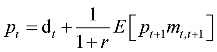
If an economy has no arbitrage, the martingale representation of Harrison and Kreps [1] and Harrison, Pliska [8] implies that an asset price can be written

(1)

where are the cashflows and is a stochastic discount factor (SDF)¹. This says that the value of a claim can be decomposed into the payments and a covariance term.

If the asset price is a binomial process (or diffusion), the one-step ahead conditional variance is

(2)

Combining Equations (1) and (2), the conditional variance of the RHS of Equation (1) must also be positive. Thus under no arbitrage, either the payout or the SDF (or both) must also be risky each period.

For the purposes valuing contingent claims, this complicates the interpretation and application of classical methods². Black and Scholes [2] assume the underlying stock price is a diffusion process. It is continuously risky (the instantaneous variance is positive). This means the LHS of Equation (1) has a strictly positive variance. But they also assume that there are no risky payments and no risky discounting. This would imply the RHS of Equation (1) has identically zero variance.

The full set of assumptions made in Black and Scholes [2] can be made consistent by dropping the standard no arbitrage condition. Without a no arbitrage condition, the martingale representation (1) of Harrison and Kreps [1] and Harrison and Pliska [8] needs not hold. Changes in the asset price can be divorced from both payments and discounting. For example, price moves could be driven by incomplete information or by learning about distributions of random variables.

Unfortunately, such a solution then creates another problem. If the economy violates the no arbitrage condition, we cannot use it to value contingent claims. This does not mean that they cannot be valued-rather, they cannot be valued by arbitrage methods.

We could as an alternative solution insist on keeping the no arbitrage condition and drop the classical assumptions about either dividends or discount rates. No arbitrage can be maintained if the binomial asset price is driven by binomial dividends or a binomial discount rate.

For stocks, bonds and many other assets types, it would be empirically unreasonable to assume risky payments are made every period. This leaves as the only realistic possibility allowing the discount rate to be risky every period. In this case, the asset behaves like a perpetuity. All variations in the asset price come from changes in the discount rate.

The structure of the article is as follows: Section 2 outlines the main result in discrete time using the binomial model. Section 3 analyzes the implications for continuous-time option pricing models. Some solutions are discussed in Section 4 and Section 5 concludes.

2. Risky Asset Prices under No Arbitrage

Before turning to the analysis in continuous time, we discuss the Binomial model. The discrete time analog simplifies the mathematics somewhat without any loss in intuition. If there is no arbitrage, the value of a claim can be written as an expectation

(3)

where is the payout at time t and is the 1-step ahead stochastic discount factor (SDF) at time t.

Under the no arbitrage condition (as defined by Harrison and Kreps [1]), an asset price is equal to an observed payment plus a covariance. To calculate the covariance term at any time t, all we need to know is the joint distribution of and.

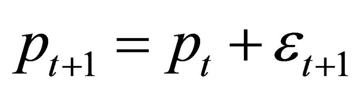
The simplest binomial asset price model is the process

(4)

where

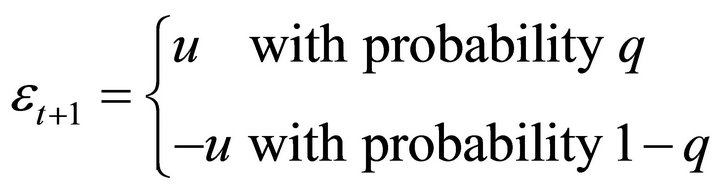
and is the step size³. Combining (3) with (4), the asset price equals

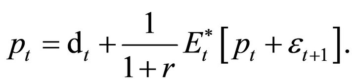
Rearranging and simplifying terms,

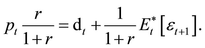
Write out the expectation,

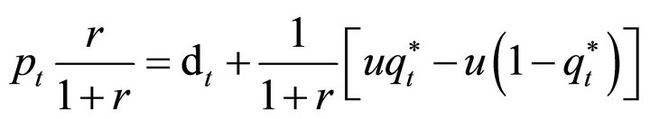(5)

where is the Arrow-Debreu state price or martingale-equivalent probability of an up move. From Harrison and Pliska [8], these subjective probabilities are given by

(6)

where q is the actual probability of an up-move and the SDF. Making this replacement in Equation (5),

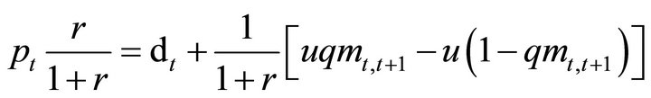
and simplifying

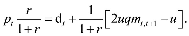(7)

We can explicitly calculate the variance of the LHS of this equation. The one-step ahead conditional variance at,

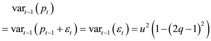
which is strictly positive for any non-degenerate Binomial. This of course implies the conditional variance

(8)

Turning to the RHS of Equation (7), the conditional variance equals

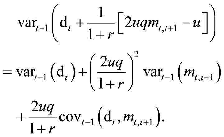(9)

If for some t, the payments and SDF were known

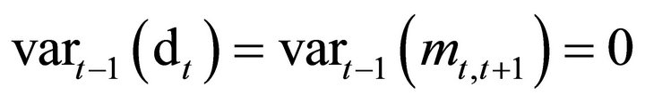(10)

expression (9) would be identically zero. Since a Binomial asset price is always risky, Equation (10) cannot hold. At least one of the two variables must be random each period so that

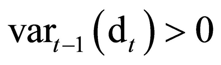or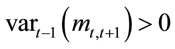

for any t.

3. Implications for Option Pricing Models

The workhorse model of asset prices in continuous-time models is the generic diffusion process

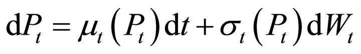(11)

where dW_t is a standard Brownian motion. The variance is determined by the function which is defined as

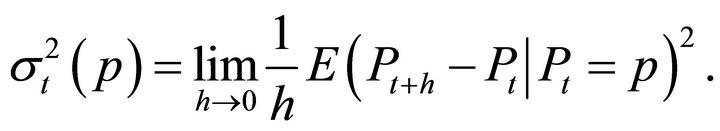
At any time t, is the instantaneous variance and the instantaneous drift.

For the diffusions typically used in Finance, including Black-Scholes [2], Cox, Ingersoll, Ross [6] and in the multivariate case, Heath, Jarrow, Morton [7] and Heston [5], the instantaneous variance is positive for all t and all P_t

(12)

There is no state of the world in which changes in price are deterministic.

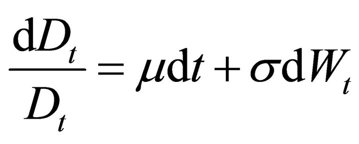
A leading example is the lognormal diffusion of BlackScholes [2],

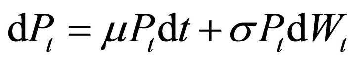(13)

where are fixed constants. The volatility parameter s must be strictly positive or the price process would be purely deterministic for all time periods. In this case, the instantaneous variance is simply

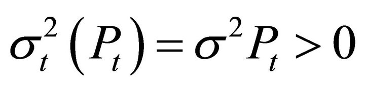(14)

and is strictly positive.

The option pricing formula originally formulated in Black and Scholes [2] is derived under the conditions:

Assumption 1. The underlying stock price P_t is a Geometric Brownian Motion.

Assumption 2. The discount rate is not stochastic.

Assumption 3. The dividend payment D_t is not stochastic over.

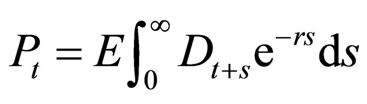
Assumptions 1-3 cannot all hold simultaneously under the no arbitrage condition defined in Harrison and Kreps [1] and Harrison and Pliska [8]. The martingale representation which results from no arbitrage implies that the price is an expectation,

(15)

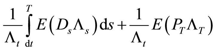
where T is any future date and L_t,t+s is the stochastic discount factor. Rearranging Equation (15),

(16)

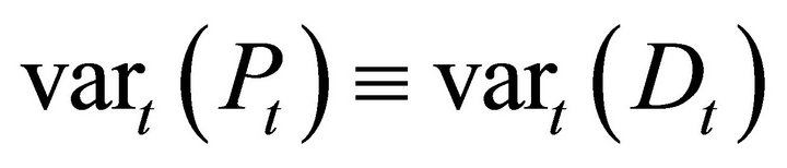
for any. The instantaneous variance of P_t is just

(17)

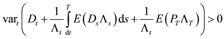
Expanding the conditional variance,

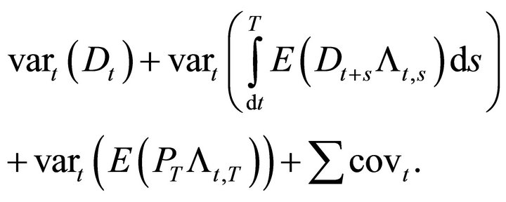(18)

Under the Black-Scholes Assumption 3, the variance of the payments are zero for. The first term in (18) is trivially zero.

Assumption 2 of Black-Scholes says the discount factors L_t,t+s also have zero variance. This implies that

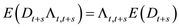
which is a known constant. The conditional variance

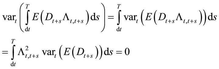
since the variance of a unconditional mean is zero. Similarly the third term in (18) is

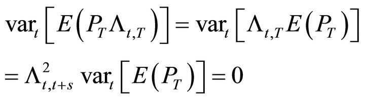(19)

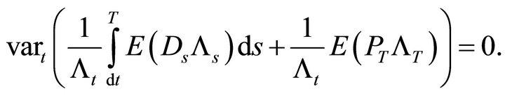
where is an unconditional mean. The covariance terms also vanish so that each element in (18) is identically zero.

We conclude that the conditional variance would be

under the standard no arbitrage condition. This contradicts Assumption 1, that the price is a diffusion process.

4. Possible Solutions

Under no arbitrage the price of an asset is driven by two fundamentals—the payments on which it is a claim and the discount rate. The Black-Scholes [2] Assumptions 1- 3 can be made consistent but only by violating no arbitrage.

Intuitively, Black-Scholes [2] construct a stock price that is continuously risky but for no fundamental reason—not because of risky payments nor because of changes in discounting. We can imagine, for example, that unpredictable stock moves are driven by incomplete information or by learning about distributions of random variables. Learning allows the stock price to be de-coupled from the fundamentals, in the manner of Assumptions 1-3. But this comes at the cost of violating the no arbitrage condition.

This is an important consideration. If the economy violates no arbitrage, we can no longer use it to value derivatives. Without some additional restriction, it is not necessarily true that the value of a contingent claim will depend on its underlying.

Since the stock does not depend on its underlying (the dividends), it would seem unnatural to assume that an option or other contingent claim would depend on its underlying (the stock). Nevertheless, we could follow the original Black-Scholes [2] development and explicitly add a condition like:

Assumption 4. The value of an option depends on its underlying asset price and not on any other random variables.

However, Assumption 4 cannot be made consistent with a no arbitrage condition. Rather it must replace the no arbitrage condition, since Assumptions 1-3 imply no arbitrage is violated.

We could also examine what would happen if we drop the assumptions about either dividends or discount rates. Continue to assume that the underlying asset price is a Geometric Brownian motion. First, make no assumption about the dividend payments, but suppose the discount rate is not stochastic.

From (16), the instantaneous variance of the underlying price is

(20)

which is strictly positive for all. The second and third terms in expression (17)

(21)

contain only constants and unconditional moments. The variance of an unconditional moment is zero so that

The only term that remains is D_t as the sole source of risk. It follows that

all variance in the asset price is explained by the risky dividend.

This would hold, for example, with dividends that are proportional to the stock price, 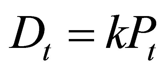where k is some constant. This implies D_t is linear in P_t and in particular that the dividend process D_t is also a lognormal diffusion (this follows immediately from Ito’s Lemma).

Since the instantaneous variance of the dividend is positive, the discount rate must be constant if we want to use arbitrage pricing. The asset price would in this case equal

where r is the constant discount rate. Since

we can write the price

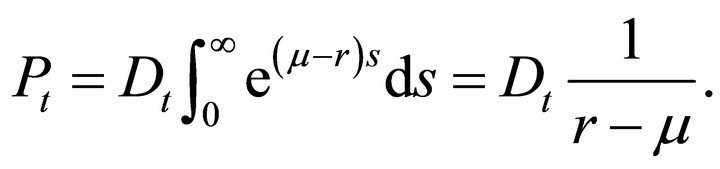
The stock is a linear derivative written on the dividend payment and obeys a form of the Gordon growth model for stock prices. This may be an unrealistic characterization of dividend payments at high frequency such as daily observations.

Risky Discounting

Suppose that instead of deriving the behavior of dividends, we assume dividends are deterministic

(22)

but we make no assumptions about discount rates.

The variance of the asset price is thus given by the last two terms in (18). The instantaneous variance is

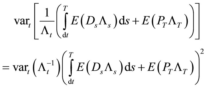(23)

where we have taken the unconditional moments out of the variance. Expression (20) is positive if and only if

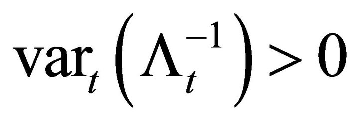(24)

the discount rate is stochastic at any time t.

5. Conclusions

If an asset price is modeled using binomial trees or their continuous-time diffusion limits, it is risky each period. A standard no arbitrage condition implies that there must also be a risky dividend and/or risky discount rate each period.

In order to value derivatives on an asset by arbitrage, we cannot allow both to be risky simultaneously. This leaves two possibilities. We can treat the dividends as a diffusion and fix the discount rate. This would seem somewhat unrealistic for most asset types such as stocks whose dividends tend to be smooth and paid only intermittently. Alternatively, we can assume dividends are purely deterministic and let the discount rate be a diffusion.

Another possibility is to abandon arbitrage valuation of contingent claims in favor of other methods (e.g., Heston [5]) which can accommodate multiple risky shocks. This would permit modeling both the discount rate and the dividend payment as risky simultaneous.

6. Acknowledgements

I am grateful to Peter Christoffersen, Tom George and Larry Samuelson for their comments. Any errors or inaccuracies are mine.

REFERENCES

NOTES

¹We follow Cox and Rubinstein [9] in using the term “binomial process” to refer generally to two-state models in discrete time. This encompasses models in which the log of the stock price at any time period has a binomial distribution. The convergence of binomial models to diffusion limits is formally studied in Brennan and Schwartz [10], Cox, Ross and Rubinstein [11], Duffie and Protter [12] and He [13].

²Note that this problem cannot be illustrated in model with less than 3 periods, as Equation (1) is ill-defined if T < 3. In this sense, there is a strong loss-of-generality is describing the continuous-time framework with a 2-period model as is commonly done in textbook expositions of option-pricing.

³This discussion is not sensitive to the particular functional form of the two-state Binomial model. The analysis would be virtually identical, for example, if the price was a geometric Brownian motion,

REFERENCES

- J. M. Harrison and D. M. Kreps, “Martingales and Arbitrage in Multiperiod Securities Markets,” Journal of Economic Theory, Vol. 20, No. 3, 1979, pp. 381-408. doi:10.1016/0022-0531(79)90043-7
- F. Black and M. Scholes, “The Pricing of Options and Corporate Liabilities,” Journal of Political Economy, Vol. 81, No. 3, 1973, pp. 637-659. doi:10.1086/260062
- R. C. Merton, “The Theory of Rational Option Pricing,” Bell Journal of Economics and Management Science, Vol. 4, No. 1, 1973, pp. 141-183. doi:10.2307/3003143
- A. Melino and S. Turnbull, “Pricing Foreign Currency Options with Stochastic Volatility,” Journal of Econometrics, Vol. 45, No. 1-2, 1990, pp. 239-265. doi:10.1016/0304-4076(90)90100-8
- S. Heston, “A Closed-Form Solution for Optoins with Stochastic Volatilityi with Applications to Bond and Currency Options,” Review of Financial Studies, Vol. 6, No. 2, 1993, pp. 327-344. doi:10.1093/rfs/6.2.327
- J. C. Cox, J. E. Ingersoll and S. A. Ross, “A Theory of the Term Structure of Interest Rates,” Econometrica, Vol. 53, No. 2, 1985, pp. 385-408. doi:10.2307/1911242
- D. Heath, R. Jarrow and A. Morton, “Bond Pricing and the Term Structure of Interest Rates: A New Methodology for Contingent Claims Valuation,” Econometrica, Vol. 60, No. 1, 1992, pp. 77-106. doi:10.2307/2951677
- J. M. Harrison and S. Pliska, “Martingales and Stochastic Integrals in the Theory of Continuous Trading,” Stochastic Processes and Their Applications, Vol. 11, No. 3, 1981, pp. 215-260. doi:10.1016/0304-4149(81)90026-0
- J. C. Cox and M. Rubinstein, “Options Markets,” Prentice-Hall, Upper Saddle River, 1985.
- M. J. Brennan and E. S. Schwartz, “Finite Difference Methods and Jump Processes Arising in the Pricing of Contingent Claims: A Synthesis,” Journal of Financial and Quantitative Analysis, Vol. 13, No. 3, 1978, pp. 461-474. doi:10.2307/2330152
- J. C. Cox, S. A. Ross and M. Rubinstein, “Options Pricing: A Simplified Approach,” Journal of Financial Economics, Vol. 7, No. 3, 1979, pp. 229-263. doi:10.1016/0304-405X(79)90015-1
- J. D. Duffie and P. Protter, “From Discrete to Continuous Time Finance: Weak Convergence of the Financial Gain Process,” Stanford University, Stanford, 1988.
- H. He, “Convergence from Discrete to Continuous Time Contingent Claim Prices,” Review of Financial Studies, Vol. 3, No. 4, 1990, pp. 523-546. doi:10.1093/rfs/3.4.523
NOTES
1We follow Cox and Rubinstein [9] in using the term “binomial process” to refer generally to two-state models in discrete time. This encompasses models in which the log of the stock price at any time period has a binomial distribution. The convergence of binomial models to diffusion limits is formally studied in Brennan and Schwartz [10], Cox, Ross and Rubinstein [11], Duffie and Protter [12] and He [13].
2Note that this problem cannot be illustrated in model with less than 3 periods, as Equation (1) is ill-defined if T < 3. In this sense, there is a strong loss-of-generality is describing the continuous-time framework with a 2-period model as is commonly done in textbook expositions of option-pricing.
3This discussion is not sensitive to the particular functional form of the two-state Binomial model. The analysis would be virtually identical, for example, if the price was a geometric Brownian motion,