American Journal of Operations Research
Vol.3 No.1A(2013), Article ID:27554,9 pages DOI:10.4236/ajor.2013.31A018
Complex Networks: Traffic Dynamics, Network Performance, and Network Structure
1School of Electrical & Computer Engineering, The University of Oklahoma, Tulsa, USA
2Department of Computer Science, The University of Oklahoma, Norman, USA
Email: ziping.hu@ou.edu, thulasi@ou.edu, pverma@ou.edu
Received December 2, 2012; revised January 8, 2013; accepted January 17, 2013
Keywords: Complex Networks; Betweenness Centrality; Network Polarization; Average Path Length; Throughput; Delay; Packet Loss
ABSTRACT
This paper explores traffic dynamics and performance of complex networks. Complex networks of various structures are studied. We use node betweenness centrality, network polarization, and average path length to capture the structural characteristics of a network. Network throughput, delay, and packet loss are used as network performance measures. We investigate how internal traffic, through put, delay, and packet loss change as a function of packet generation rate, network structure, queue type, and queuing discipline through simulation. Three network states are classified. Further, our work reveals that the parameters chosen to reflect network structure, including node betweenness centrality, network polarization, and average path length, play important roles in different states of the underlying networks.
1. Introduction
In network science, complex systems are described as networks consisting of vertices and interactions or connections among them. Many social, biological, and communication systems are complex networks. The study of structural and dynamical properties of complex networks has been receiving a lot of interests. One of the ultimate goals of the studies is to understand the influence of topological structures on the behaviors of various complex networks, for instance, how the structure of social networks affects the spread of diseases, information, rumors, or other things; how the structure of a food web affects population dynamics; how the structure of a communication network affects traffic dynamics, and network performance such as robustness, reliability, traffic capacity, and so on.
There is a wealth of literature focusing on traffic dynamics and different performance aspects of communication networks. A basic model, which is aimed at simulating a general transport process on top of a communication network, has been proposed by Ohira and Sawatari [1]. It demonstrates that network traffic exhibits a phase transition from free flow to congestion as a function of packet generation rate. The model has been generalized in various ways [2-12] for the study of different communication networks. The authors in [2-3] investigate congestion phenomena in complex communication networks by implementing traffic-aware routing schemes in the model. Much research has focused on scale-free (SF) networks because of the discovery of power-law degree distribution of many real-world networks [13-14]. Due to the structural properties of SF networks, different routing strategies [4-11] are proposed in order to improve traffic capacity of these networks. Since lattice networks are widely used in distributed parallel computation, distributed control, satellite constellations, and sensor networks, Barrenetxea, Berefull-Lozano, and Vetterli [12] have studied the effect of routing on the queue distribution, and investigated the routing algorithms in lattice networks that achieve the maximum rate per node under different communication models.
The work of Tizghadam and Leon-Garcia [15-17] focuses on the robustness of communication networks. They introduce the notion of network criticality. They find that network criticality directly relates to network performance metrics such as average network utilization and average network cost. In addition, by minimizing network criticality, the robustness of a communication network can be improved. In order to measure nodal contribution to global network robustness, Feyessa and Bikdash [18] have made comparison among different centrality indices. For the design of reliable communication networks, Hu and Verma [19] propose a heuristic topology design algorithm that can effectively improve network reliability. In [20], we have investigated the latency of SF networks and random networks under different routing strategies. In a recent work [21], we have explored the influence of network structure on traffic dynamics in complex communication networks.
In this paper, we investigate how internal traffic, throughput, delay, and packet loss change as a function of packet generation rate, network structure, queue type, and queuing discipline through simulation. Four different types of networks are chosen as the underlying networks because of their distinct structural features. They are the SF network, the random network, the ring lattice (RL) network, and the square lattice (SL) network. We use node betweenness centrality, network polarization, and average path length, to capture the structural features of the networks.
Based on observed traffic dynamics in the networks studied, we classify three network states: traffic free flow state, moderate congestion state, and heavy congestion state. Simulation results indicate that during each different state, the structural differences among the underlying networks play important roles in the performance of these networks. Through the work, we shall gain deep insights on the dependency of network performance on the structural properties of networks, which could help in designing better network structures and better routing protocols.
The paper is organized as follows. Section II presents our network model. Simulation results and analysis are provided in Section III. Section IV concludes the work.
2. Network Model
Four different types of networks are chosen as the underlying networks. They are the SF network, the random network, the SL network, and the RL network. One of their structural differences lies in their distinct nodal degree distributions. The degree of a node is the total number of links connecting it. The SF network is built based on the Barabasi-Albert (BA) model proposed in [13]. It has a power law degree distribution so that most nodes have very low degrees, but a few nodes (called hubs) could have extremely high degrees. The random network is formed according to the Erdős-Rényi (ER) model proposed in [22]. The random ER network follows Poisson degree distribution when network size is large; therefore, the degrees of most nodes are around the mean degree. In the SL network, all the nodes except those located on the edge of the square have the same degree. The RL network is constructed by connecting each node on a circle to its  nearest neighboring nodes. Apparently, all the nodes in the RL network have the same degree.
In the paper, we use node betweenness centrality, network polarization, and average path length to capture the structural characteristics of above networks. The node betweenness Bi for a node i is defined here as the total number of shortest path routes passing through that node. Nodes with high betweenness values participate in a large number of shortest paths. Therefore, initial congestion usually happens at nodes of the highest betweenness value. Node betweenness reflects the role of a node in a communication network. Normally, high betweenness nodes also have high degrees. The node betweenness distribution of a communication network is demonstrated through a measure of the polarization, π, of the network [23]. It is defined as:
 (1)
(1)
where Bmax is the maximum betweenness value, is the average betweenness value. We find that π as an indication of node betweenness distribution suits our work better than others (e.g. standard deviation). The large polarization value of a network tells us that at least one node possesses much larger betweenness values than most of the other nodes in the network. Therefore, the larger the value π is, the more heterogeneous the network is. On the other hand, for very homogeneous networks, π is very small. For example, for the RL network, we have π ≈ 0. The average path length of a network is defined as the average of the shortest path lengths among all the source-destination pairs. In the next section, we are going to demonstrate how node betweenness, network polarization, and average path length relate to the performance of the underlying networks.
The above three parameters capture the structural features of a network from different angles. They are also interrelated. Usually, the more heterogeneous (larger π, or relatively higher Bmax) the network is, the shorter the average path length is. The reason is that high betweenness nodes (usually hubs) serve as shortcuts for connecting node pairs. In addition, the following relationship between shortest path length and node betweenness centrality can be easily found,
 (2)
(2)
where Dij stands for the shortest path length from node i to node j, Bi stands for the betweenness value of node i.
In the underlying networks studied, fixed shortest path routing strategy is implemented. The length of the shortest path is the minimum hop count between a sourcedestination pair. Given network topology, each node calculates the shortest paths to all the other nodes using Dijkstra’s algorithm. Then a routing table is constructed at each node. A routing table contains three columns: destination node, next node to route a packet to the destination, and the hop count to the destination.
The model used to govern the dynamic processes of packet generation, storage, and routing is similar to the model by Ohira and Sawatari [1]. In [1], only infinite queues and first-in-first-out (FIFO) queuing discipline are implemented; while in our model, we include also finite queues and last-in-first-out (LIFO) queuing discipline. Especially, the implementation of finite queues is close to real-world scenarios. In the model, we assume that time is slotted. During each time slot, first, packets are generated at each node with the rate λ, the destination of a packet is randomly chosen among all other nodes. Each node is endowed with a queue in which packets are stored waiting to be processed. Then, if the queue is not empty, each node transmits one packet from its queue to one of its neighbors according to its routing table. When a packet reaches its destination, it is eliminated from the system. The traffic load on a node is quantified by the number of packets stored in its queue waiting to be processed.
In the paper, we study traffic dynamics and network performance as a function of packet generation rate, network structure, queue type, and queuing discipline. We use throughput, average packet delay, and packet loss as main performance measures. Throughput is defined as the average number of delivered packets per time slot. The average packet delay is defined as the average time that a delivered packet spent in the network. Under heavy traffic load, packet loss is defined as the average number of discarded packets per time slot. Packet loss is caused by traffic overflow at nodes with heavy traffic; thus, it is evaluated only when finite queues are implemented.
3. Simulation Results and Analysis
In the simulation, a discrete time clock k is used. Simulation starts with k = 0, for each passed time slot, k is incremented by 1. The performance of an underlying network is measured by its throughput o(k), average packet delay τ(k), and packet loss l(k). The values of o(k), τ(k), and l(k) are calculated respectively as the average from the start of simulation (k = 0) to time k. We use n(k) to represent the total number of packets within the network at time k.
In the simulation, the underlying networks are generated with approximately the same number of nodes and links. The SF network, the random ER network, and the RL network are all generated with 50 nodes and 100 links. The SL network is generated with 49 nodes and 84 links because of its structural restrictions. Four different cases are considered: infinite queues with FIFO queuing discipline, infinite queues with LIFO queuing discipline, finite queues with FIFO queuing discipline, and finite queues with LIFO queuing discipline. Then, we investigate network performance as a function of λ in above four different cases. Three network states are identified accordingly. We demonstrate that how, in different network states, the structure of a network influences its performance.
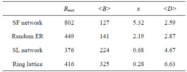
Table 1 lists the related parameters of the underlying networks. It tells us that the RL network has the lowest polarization value π, which shows its almost homogeneous structure in terms of node betweenness distribution; while the SF network has the highest π, which demonstrates its most heterogeneous structure. In addition, the RL network has the longest average path length
3.1. Total Internal Traffic n(k)
In this section, by investigating the change of n(k) as a function of packet generation rate λ, we reproduce network phase transition reported in [1-3]. Simulation results are plotted in Figure 1. From Figure 1, we observe that the change of n(k) as a function of packet generation rate is independent of queuing discipline, but depends heavily on queue type. It is shown in Figures 1(a) and (c) that when queue size is infinite, a critical point λc is observed in all these networks where a network phase transition takes place from traffic free flow to congestion. Compared with Figures 1(a) and (c), it is shown in Figures 1(b) and (d) that when queue size is finite, the abrupt change of internal traffic at the critical points is greatly smoothed.
When , a network is in steady state or traffic free flow state. In this sate, n(k) remain slow and almost unchanged with the increase in incoming traffic λ. According to Little’s law, for a network of size N, the number of packets created per unit time (given by N × λ) must be equal to the number of packets delivered per time slot. The number of delivered packets per time slot is
Table 1. Network parameters
 , hence
 . However, n(k) is proportional to the average path length of the networks. For instance, the RL network has the most internal traffic because it has the longest average path length.
From Figures 1(a) and (c), we observe that compared with the other networks, the SF network has the lowest value of λc. The reason lies in its highest Bmax among all the networks studied. According to the definition of node betweenness centrality, the node with maximum betweenness value Bmax handles the heaviest traffic because it participates in the largest number of shortest path routes. With increasing incoming traffic, initial congestion (or quick accumulation of packets) shall take place first at the node with Bmax. In a similar way, the SL network obtains highest λc because it has the lowest Bmax. Thus, the critical point λc of a network is inverse proportional to its Bmax.
When , the networks enter into congestion state, where n(k) start increasing quickly with the increase in λ in the infinite queue case (shown in Figures 1(a) and (c)). However, in the finite queue case, we observe from Figures 1(b) and (d) that, the change of n(k) is greatly smoothed. Especially, the curve that represents the change of n(k) in the SF network is the most flat among the four networks. The reason lies in that the few high betweenness nodes are quickly congested in the SF network; therefore, the huge amount of traffic that goes through those nodes has to be discarded because the queue size is finite. With the increase in λ, n(k) does not change much. However, since the incoming traffic is not yet very heavy, for the RL network, packets start to accumulate at almost all the nodes because of its homogeneous structure, which leads to relatively quick increase in its internal traffic n(k).
3.2. Network Throughput o(k)
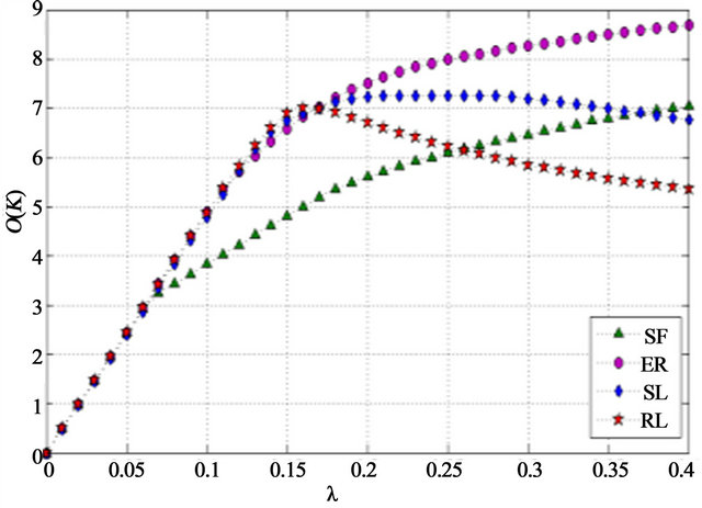
This section investigates network throughput as a function of packet generation rate, network structure, queue type, and queuing discipline. Simulation results are plotted in Figures 2 and 3. inf. stands for infinite queue type. fin. stands for finite queue type.
From Figure 2, we observe that network throughput is almost independent of queue type and queuing discipline, but depends heavily on the structure of the underlying networks. Figure 2 shows that when , with the increase in packet generation rate λ, network throughput increases linearly, which demonstrate that the networks are in traffic free flow state. When λ exceeds the critical point λc, the increase in network throughput becomes slower because packets start to accumulate in the networks. We say that a network is in moderate congestion
 (a)
(a)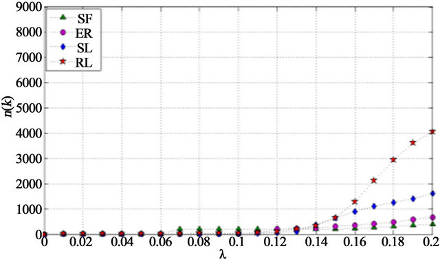 (b)
(b)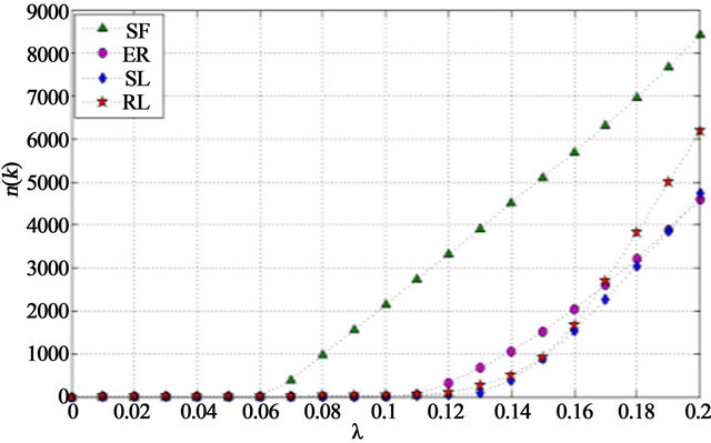 (c)
(c)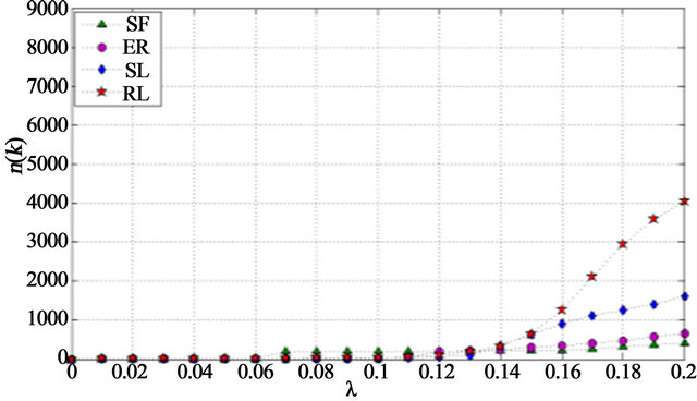 (d)
(d)
Figure 1. n(k) as a function of λ (k = 2000): (a) Infinite queue, FIFO; (b) Finite queue, FIFO; (c) Infinite queue, LIFO; (d) Finite queue, LIFO.
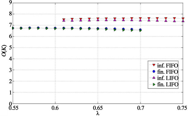
state. With further increase in λ, we observe clearly from Figure 2 that the throughput of the SL network and the RL network quickly drops. Figure 3 displays the throughput of the SF network and the random ER network under different queue types and queuing disciplines when the incoming traffic is very heavy. From Figure 3, a similar phenomenon is found in the SF network and the random ER network, even though the drop in network throughput is much slower. When network throughput starts to drop, we say that a network has entered into heavy congestion state.
When a network enters into moderate congestion state, at least one node is congested. From Figure 2, we observe that the SF network is the first that enters into moderate congestion state because it has the highest Bmax. Compared with the others, the performance of the SF network is the worst. The reason lies in its most heterogeneous structure (largest π). When the SF network is in moderate congestion state, huge amount of packets quickly accumulate at one or several nodes of extremely high betweenness values when many other nodes are idle (or do not have enough packets to send). A similar phenomenon is observed in the random ER network, but the random ER network performs much better than the SF network because of its much smaller polarization value π. According to the same reasoning, we find that during moderate congestion state, both the RL network and the SL network achieve a little higher throughput than the other two because of their lower polarization value π. However, from Figures 2 and 3, we observe that both the RL network and the SL network have much shorter moderate congestion duration before entering into heavy congestion state.
We find that even though in moderate congestion state, congestion happens at only a few nodes, network throughput depends heavily on traffic load distribution. The less the value of network polarization is, the more homogeneous (in terms of node betweenness distribution) a network is, and the more balanced the traffic load is distributed; therefore, the better the network performs. For the RL network and the SL network, their almost uniform node betweenness distribution results in more balanced traffic load distribution among all the nodes so that many packets are delivered successfully. Therefore, we may say that in moderate congestion state when traffic is not yet very heavy, network throughput strongly relates to network polarization.
When λ increases beyond a specific value (this value is different for different networks), the networks enter into heavy congestion state. In this state, more nodes in the networks are congested. We observe that the smaller the network polarization is, the faster the network enters into heavy congestion state (shown in Figure 2). In this state, network throughput starts to decrease. For the SF net
 (a)
(a) (b)
(b)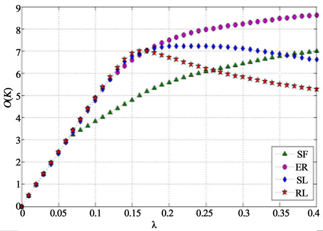 (c)
(c)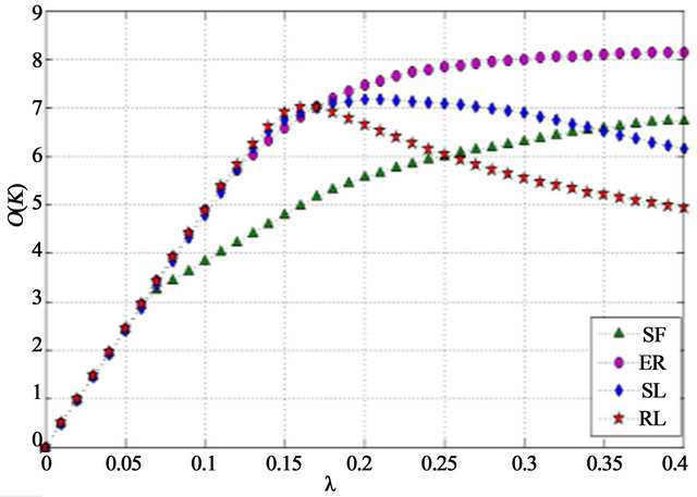 (d)
(d)
Figure 2. o(k)as a function of λ (k = 2000): (a) Infinite queue, FIFO; (b) Finite queue, FIFO; (c) Infinite queue, LIFO; (d) Finite queue, LIFO.
work and the random ER network, because of their heterogeneous structure (large π), even though most traffic is jammed at more nodes of high betweenness values, a small amount of traffic bypassing those congested nodes can still be delivered successfully. Compared with the SF network, the performance of the random ER network is much better because the random ER network is relatively less heterogeneous (relatively smaller π). For the RL network and the SL network, their structure is more homogeneous. However, when the incoming traffic becomes very heavy, their very long average path length causes huge amount of internal traffic. In addition, since their node betweenness distribution is almost uniform and their average betweenness value is high, almost all the nodes are congested (few packets can be delivered successfully). Compared with the RL network, the SL network performs better because of its relatively shorter average path length and lower betweenness values. Therefore, in heavy congestion state, average path length, node betweenness, and node betweenness distribution all play important roles in network throughput.
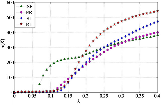
3.3. Average Packet Delay τ(k)
Average packet delay as a function of packet generation rate, network structure, queue type, and queuing discipline is investigated in this section. Simulation results are plotted in Figure 4.
In traffic free flow state , we know that all the networks perform the same in terms of throughput (throughput increases linearly with λ), but it is not so in terms of average packet delay. In traffic free flow statefrom
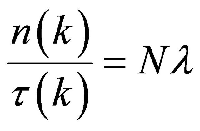 , we obtain
 . Since n(k)
depends on the average path length of a network, the average packet delay τ(k) also depends on the average path length of the network. It is verified through our simulation. For instance, the SF network displays the lowest τ(k) because it has the shortest average path length. Therefore, in traffic free flow state, the average path length plays a major role in average packet delay of the networks.
When the networks enter into moderate congestion state, from Figure 4, we find that the average delay performance relies heavily on queue type and queuing discipline. When LIFO queuing discipline is implemented, the average packet delay of all the networks reaches the lowest (shown in Figures 4(c) and (d)). This phenomenon is easy to understand. From Figures 4(a) and (b), when FIFO queuing discipline is implemented, an abrupt increase in average packet delay is observed in all the networks. In addition, the average packet delay is greatly influenced by queue types and network structure (shown in Figures 4(a) and (b)). For instance, when the SF net-
 (a)
(a) (b)
(b)
Figure 3. o(k) as a function of λ (k = 2000): (a) The SF network; (b) The random ER network.
work and the ER network are in moderate congestion state but the SL network and the RL network are already in heavy congestion state, the average delay of the SL network and the RL network is higher because of their longer average path length.
The analysis made in above sections is also verified by our observation on the changes in queue length (total number of packets in a queue) through simulation. In traffic free flow state (we choose λ = 0.05), most queues in all the networks are almost empty. In moderate congestion state (we choose λ = 0.13), most queues in the RL network contain several packets, a few queues contain several tens of packets, and the length of one queue exceeds one hundred packets. It is similar for the SL network. Most queues in the random ER network are almost empty, but the queues at a few nodes of high betweenness values contain hundreds of packets. Similar to the random ER network, most queues in the SF network are almost empty, but two queues at two nodes of extremely high betweenness values contain thousands of packets respectively. In heavy congestion state (a different λ is chosen for each network), for the RL network, the whole network is congested (most queues contain several tens of packets, a few queues contain even hundreds of pack-
 (a)
(a)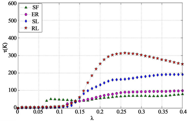 (b)
(b)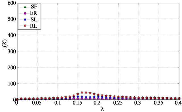 (c)
(c)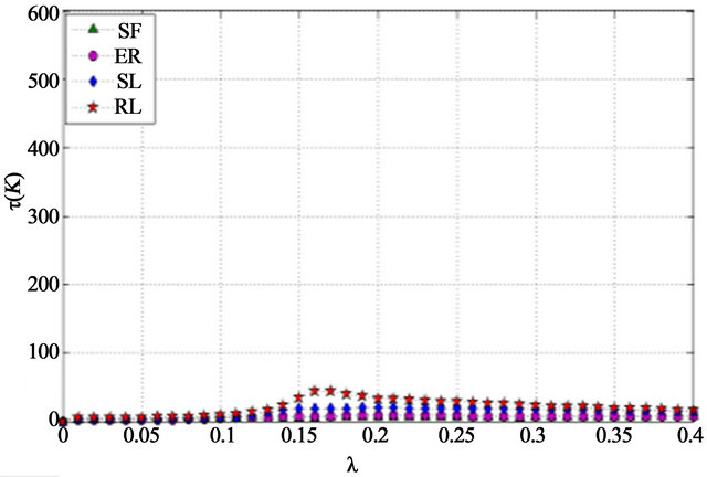 (d)
(d)
Figure 4. τ(k) as a function of λ (k = 2000): (a) Infinite queue, IFO; (b) Finite queue, FIFO; (c) Infinite queue, LIFO; (d) Finite queue, LIFO.
ets). It is similar to the SL network. While for the random ER network and the SF network, even though more nodes of high betweenness values are heavily congested, about half of the queues are still almost empty. Interestingly, we find that no matter what the structure of an underlying network is, congestion always takes place when a large number of packets start to accumulate at a few nodes.
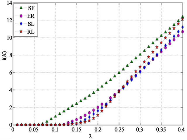
3.4. Packet Loss l(k)
This section investigates the average packet delay as a function of packet generation rate, network structure, queue type, and queuing discipline. Simulation results are plotted in Figure 5. Since traffic overflow happens only when finite queues are implemented, packet loss is evaluated in two cases: finite queues with FIFO queuing discipline and finite queues with LIFO queuing discipline.
Figure 5 clearly shows that only when the networks enter into congestion state, packet loss starts to increase abruptly. It also shows that packet loss depends on incoming traffic and network structure, but is independent of queuing discipline. The SF network has the highest packet loss under the same incoming traffic because large amount of traffic have to pass through a few congested nodes (hubs). The RL network achieves the lowest packet loss in moderate congestion state, but when it enters into heavy congestion state, its packet loss exceeds that of the SL and the random ER network. The reason lies in its homogeneous structure. In moderate congestion state when the incoming traffic is not yet very heavy, traffic load distributes almost uniformly in the RL network; while in heavy congestion state when the incoming traffic is heavy, its homogeneous structure, together with its long average path length, and relatively high betweenness value, leads to the congestion of the whole network.
4. Conclusion
We have investigated how internal traffic, throughput, average packet delay, and packet loss change as a function of packet generation rate, network structure, queue type and queuing discipline. Networks of various structures have been chosen as underlying networks. Based on network performance, three network states have been classified: traffic free flow state, moderate congestion state, and heavy congestion state. Under fixed shortest path routing, we have found that node betweenness centrality, network polarization, and average path length all play important roles in different states of the underlying networks. In traffic free flow state, average path length plays the major role; it directly affects average packet delay. In moderate congestion state and heavy congestion state, both average path length and node betweenness
 (a)
(a)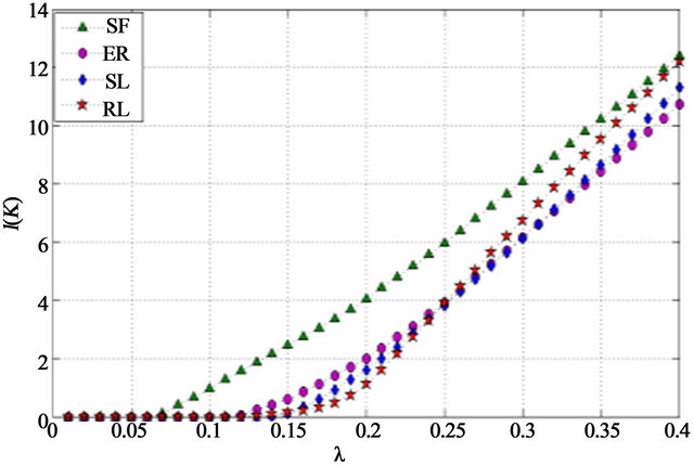 (b)
(b)
Figure 5. l(k) as a function of λ (k = 2000): (a) FIFO; (b) LIFO.
distribution play important roles in network performance. Our work could help in designing better network structures and better routing protocols.
REFERENCES
- T. Ohira and R. Sawatari, “Network Phase Transition in Computer Network Traffic Model,” Physics Review E, Vol. 58, No. 1, 1998, pp.193-195. http://dx.doi.org/10.1103/PhysRevE.58.193
- D. Martino, L. Dall’Asta, G. Bianconi and M. Marsili, “Congestion Phenomena on Complex Networks,” Physics Review E, Vol. 79, No. 1, 2009, Article ID: 015101.
- P. Echenique, J. Gomez-Gardenes and Y. Moreno, “Dynamics of Jamming Transitions in Complex Networks,” Europhysics Letters, Vol. 71, No. 2, 2005, pp. 325-331.
- Z. Jiang and M. Liang, “An Efficient Weighted Routing Strategy for Scale-Fee Networks,” Modern Physics Letters B, Vol. 26, No. 29, 2012, Article ID: 1250195. http://dx.doi.org/10.1142/S0217984912501953
- Z.-H. Guan, L. Chen and T.-H. Qian, “Routing in ScaleFree Networks Based on Expanding Betweeness Centrality,” Physica A: Statistical Mechanics and Its Applications, Vol. 390, No. 6, 2011, pp. 1131-1138.
- X.-G. Tang, E. W. M. Wong and Z.-X. Wu, “Integrating Network Structure and Dynamic Information for Better Routing Strategy on Scale-Free Networks,” Physica A: Statistical Mechanics and Its Applications, Vol. 388, No. 12, 2009, pp. 2547-2554.
- J. W. Wang, L. L. Rong and L. Zhang, “Routing Strategies to Enhance Traffic Capacity for Scale-Free Networks,” The IEEE International Conference on Intelligent Computation Technology and Automation, 2008, pp. 451-455.
- M. Tang, Z. H. Liu, X. M. Liang and P. M. Hui, “SelfAdjusting Routing Schemes for Time-Varying Traffic in Scale-Free Networks,” Physical Review E, Vol. 80, No. 2, 2009, Article ID: 026114.
- M. Tang and T. Zhou, “Efficient Routing Strategies in Scale-Free Networks with Limited Bandwidth,” Physical Review E, Vol. 84, No. 2, 2011, Article ID: 026116.
- S. Sreenivasan, R. Cohen, E. Lopez, Z. Toroczkai and H. E. Stanley, “Structural Bottlenecks for Communication in Networks,” Physical Review E, Vol. 75, 2007, Article ID: 036105.
- X. Ling, M. Hu, R. Jiang and Q. Wu, “Global Dynamic Routing for Scale-Free Networks,” Physics Review E, Vol. 81, No. 1, 2010, Article ID: 016113.
- G. Barrenetxea, B. Berefull-Lozano and M. Vetterli, “Lattice Networks: Capacity Limits, Optimal Routing, and Queuing Behavior,” IEEE/ACM Transactions on Networking, Vol. 14, No. 3, 2006, pp. 492-505. http://dx.doi.org/10.1109/TNET.2006.876187
- A.-L. Barabási and R. Albert, “Emergence of Scaling in Random Networks,” Science, Vol. 286, No. 5439, 1999, pp. 509-512. http://dx.doi.org/10.1126/science.286.5439.509
- M. Faloutsos, P. Faloutsos and C. Faloutsos, “On the Power-Law Relationships of the Internet Topology,” Computer Communication Review, Vol. 29, No. 4, 1999, pp. 41-51. http://dx.doi.org/10.1145/316194.316229
- A. Tizghadam and A. Leon-Garcia, “Robust Network Planning in Non Uniform Traffic Scenarios,” In: Computer Communications, Elsevier, Amsterdam, 2011
- A. Tizghadam and A. Leon-Garcia, “On Traffic-Aware Betweenness and Network Criticality,” Proceedings of IEEE INFOCOM, San Diego, 15-19 March 2010.
- A. Tizghadam and A. Leon-Garcia, “A Graph Theoretical Approach to Traffic Engineering and Network Control Problem,” IEEE 21st International Teletraffic Congress, Paris, 15-17 September 2009.
- T. Feyessa and M. Bikdash, “Measuring Nodal Contribution to Global Network Robusness,” Proceedings of IEEE Southeastcon, Nashville, 17-20 March 2011.
- Z. P. Hu and P. K. Verma, “Improved Reliability of FreeSpace Optical Mesh Networks through Topology Design,” Journal of Optical Communications and Networking, Vol. 7, No. 5, 2008, pp. 436-448.
- Z. P. Hu and P. K. Verma, “Impact of Network Structure on Latency in Complex Networks,” The 35th IEEE Sarnoff Symposium, Newark, 21-22 May 2012.
- Z. P. Hu and P. K. Verma, “Interplay between Traffic Dynamics and Network Structure,” The IARIA 8th International Conference on Systems, Seville, 27 January-1 February 2013.
- P. Erdős and A. Rényi, “On Random Graphs I,” Publicationes Mathematicae, Vol. 6, 1959, pp. 290-297.
- R. Guimera, et al., “Optimal Network Topologies for Local Search with Congestion,” Physics Review Letters, Vol. 89, No. 24, 2002, Article ID: 248701. http://dx.doi.org/10.1103/PhysRevLett.89.248701