18 H. N. Nguyen et al. / J. Biomedical Science and Engineering 3 (2010) 13-19
SciRes Copyright © 2010 JBiSE
1
12
1
11
() exp{()()
2
n
ii
i
mxx xx x
n
}
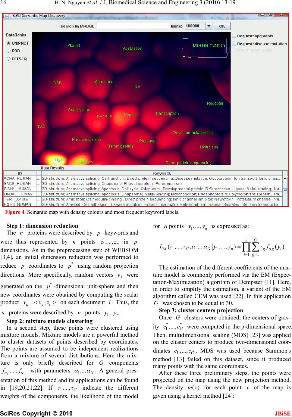
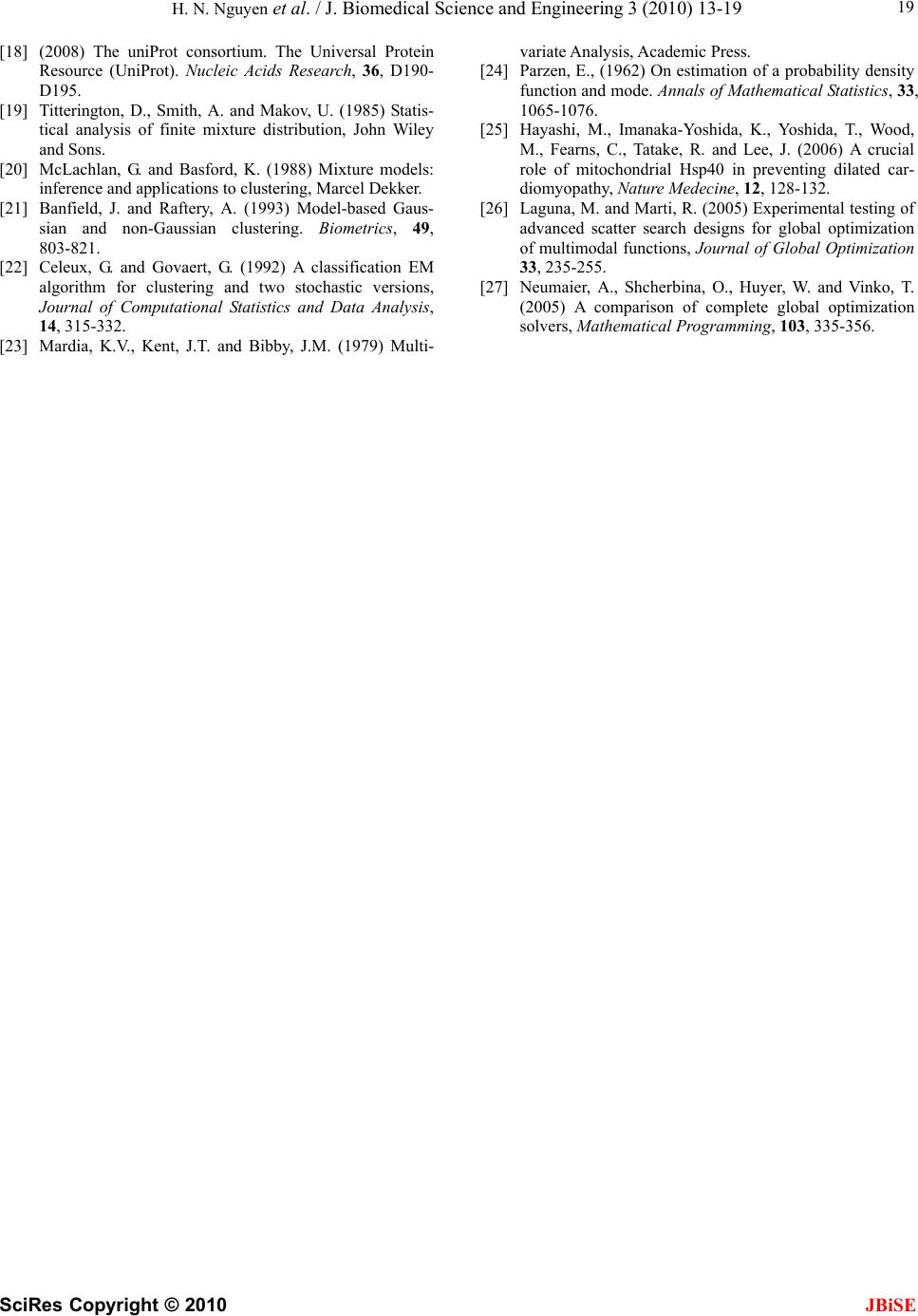
Then, a color scale ranging from purple to white, with
intermediary colors red, orange and yellow was assigned
to each point according to its density. The map is repre-
sented in Figure 4.
Then, a color scale ranging from purple to white, with
intermediary colors red, orange and yellow was assigned
to each point according to its density. The map is repre-
sented in Figure 4.
This visual representation allows a global comprehen-
sion of the whole database, which is easier to understand
than numerical or textual data. Some important key-
words shared by many proteins are visible on this map,
such as kinase, ligase and protease. At the same time,
frequent keywords, such as “complete proteome”, that
are non-informative, are avoided because they are shared
by several clusters. Another observation is that the den-
sity is far from being homogeneous, the map being more
crowded in the bottom-left corner than elsewhere.
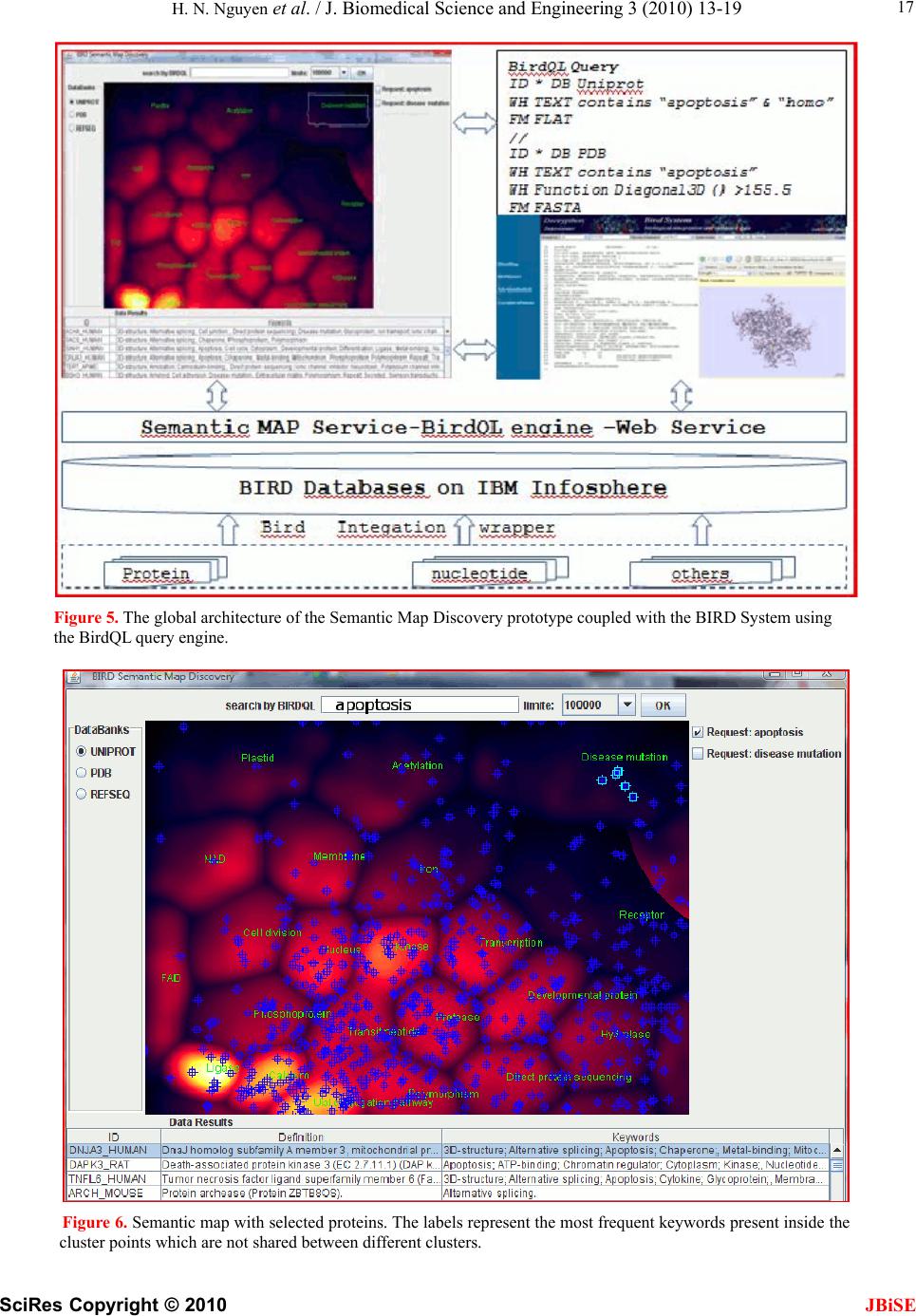
When using the integrated biological query engine
BIRD-QL of the BIRD System via a web service or http
protocol, as shown in Figure 5, the selected proteins are
represented on the maps by a plus sign of a given color.
If different selections have been performed, different
colors are used. An example is shown in Figure 6, where
proteins selected by a query with the keyword “apop-
tosis” are shown by blue plus signs. Some of these pro-
teins were selected by the user and are surrounded by a
white square. One of the proteins, DNJA3, belongs to
the small cluster labeled “disease mutation” but does not
possess the “disease mutation” keyword. Interestingly its
deficiency implies dilated cardiomyopathy [25] (MIM-
608382).
There is still room for improvement in the construc-
tion of semantic maps both at the algorithmic level and
at the software functionality level. The point’s projection
is formalized as a global optimization problem and cur-
rently, it is resolved simply using different starting points
with the Newton-Raphson method. However global op-
timization methods could also be tested [26,27]. From a
practical point of view it would also be useful to deter-
mine how many clusters or nodes are necessary to
achieve a good projection of the data points.
4. CONCLUSIONS 4. CONCLUSIONS
The main contribution of this work is a new computa-
tional solution to the construction of semantic maps. The
idea is to project points by locating them according to
cluster centers. This method can thus be coupled with
other methods such as self-organizing maps or Flexer's
approach.
The main contribution of this work is a new computa-
tional solution to the construction of semantic maps. The
idea is to project points by locating them according to
cluster centers. This method can thus be coupled with
other methods such as self-organizing maps or Flexer's
approach.
5. ACKNOWLEDGEMENTS 5. ACKNOWLEDGEMENTS
This work was supported by the CNRS, the University of Strasbourg
and the Décrypthon program initiated by the Association Française
contre les Myopathies, IBM and the CNRS. We are grateful to all
internship students who participated in this work by programming some
parts of it, namely Xavier Brotel, Jérémy Némo Trouslard and Julien
Cadet. The authors would like to thank Anne Friedrich, Laurent Philippe
Albou and Julie Thompson for helpful suggestions.
REFERENCES REFERENCES
[1] Bishop, C.M., Svens'en, M. and Williams, C.K.I. (1998)
GTM: the generative topographic mapping, Neural
Computation, 10, 215-234.
[1] Bishop, C.M., Svens'en, M. and Williams, C.K.I. (1998)
GTM: the generative topographic mapping, Neural
Computation, 10, 215-234.
[2] Lesteven, K. (1995) Multivariate data analysis applied to
bibliographical information retrieval: SIMBAD quality
control. Vistas in Astronomy, 39, 187-193
[2] Lesteven, K. (1995) Multivariate data analysis applied to
bibliographical information retrieval: SIMBAD quality
control. Vistas in Astronomy, 39, 187-193
[3] Kaski, S. (1998) Dimensionality reduction by random
mapping: Fast similarity computation for clustering,
Proceedings of IJCNN'98, International Joint Conference
on Neural Networks, IEEE Service Center, 413-418.
[3] Kaski, S. (1998) Dimensionality reduction by random
mapping: Fast similarity computation for clustering,
Proceedings of IJCNN'98, International Joint Conference
on Neural Networks, IEEE Service Center, 413-418.
[4] Lagus, K., Kaski, S. and Kohonen, T. (2004) Mining
massive document collections by the WEBSOM method.
Information Sciences, 163, 135-156.
[4] Lagus, K., Kaski, S. and Kohonen, T. (2004) Mining
massive document collections by the WEBSOM method.
Information Sciences, 163, 135-156.
[5] Chen, C. (2005) CiteSpace II: Detecting and visualizing
emerging trends and transient patterns in scientific lit-
erature. Journal of the American Society for Information
Science, 57, 359-377.
[5] Chen, C. (2005) CiteSpace II: Detecting and visualizing
emerging trends and transient patterns in scientific lit-
erature. Journal of the American Society for Information
Science, 57, 359-377.
[6] Grimmelstein, M. and Urfer, W.W. (2005) Analyzing
protein data with the generative topographic mapping
approach. innovations in classification, data science, and
information systems, Baier, D. and Wernecke, K.D.
Springer Berlin Heidelberg, 585-592.
[6] Grimmelstein, M. and Urfer, W.W. (2005) Analyzing
protein data with the generative topographic mapping
approach. innovations in classification, data science, and
information systems, Baier, D. and Wernecke, K.D.
Springer Berlin Heidelberg, 585-592.
[7] Ossorio, P.G, (1966) Classification space: a multivariate
procedure for automated document indexing and retrieval.
Multivariate Behavioral Research, 1, 479-524.
[7] Ossorio, P.G, (1966) Classification space: a multivariate
procedure for automated document indexing and retrieval.
Multivariate Behavioral Research, 1, 479-524.
[8] Deerwester, S., Dumais, S.T., Furnas, G.W., Landauer, T.
K. and Harshman R. (1990) Indexing by latent semantic
indexing. Journal of the American Society for Informa-
tion Science, 41, 391-407.
[8] Deerwester, S., Dumais, S.T., Furnas, G.W., Landauer, T.
K. and Harshman R. (1990) Indexing by latent semantic
indexing. Journal of the American Society for Informa-
tion Science, 41, 391-407.
[9] Kohonen, T. (1997) Self-Organizating Maps, Springer-
Ve rl a g.
[9] Kohonen, T. (1997) Self-Organizating Maps, Springer-
Ve rl a g.
[10] Kohonen, T. (1982) Analysis of a simple self-organizing
process. Biological Cybernetics, 44, 135-140.
[10] Kohonen, T. (1982) Analysis of a simple self-organizing
process. Biological Cybernetics, 44, 135-140.
[11] Dempster, A., Laird, N. and Rubin, D. (1977) Maximum
likelihood from incomplete data via the {EM} algorithm.
Journal of the Royal Statistical Society, Ser. B, 39,
249-282.
[11] Dempster, A., Laird, N. and Rubin, D. (1977) Maximum
likelihood from incomplete data via the {EM} algorithm.
Journal of the Royal Statistical Society, Ser. B, 39,
249-282.
[12] Flexer, A. (1997) Limitations of self-organizing maps for
vector quantization and multi-dimensional scaling. Ad-
vances in neural information processing systems, 9,
445-451.
[12] Flexer, A. (1997) Limitations of self-organizing maps for
vector quantization and multi-dimensional scaling. Ad-
vances in neural information processing systems, 9,
445-451.
[13] Sammon J.W. (1969) A non-linear mapping for data
structure analysis. IEEE Transactions on Computers, 18,
401-409.
[13] Sammon J.W. (1969) A non-linear mapping for data
structure analysis. IEEE Transactions on Computers, 18,
401-409.
[14] Bishop, C.M. and James G.D. (1993) Analysis of multi-
phase flows using dual-energy gamma densitometry and
neural networks. Nuclear Instruments and Methods in
Physics Research, Section A, 327, 580-593.
[14] Bishop, C.M. and James G.D. (1993) Analysis of multi-
phase flows using dual-energy gamma densitometry and
neural networks. Nuclear Instruments and Methods in
Physics Research, Section A, 327, 580-593.
[15] Nguyen, H., Berthommier, G., Friedrich, A., Poidevin, L.,
Ripp, R., Moulinier, L. and Poch, O. (2008) Introduction
to the new Decrypthon Data Center for biomedical data,
Proc CORIA', 32-44.
[15] Nguyen, H., Berthommier, G., Friedrich, A., Poidevin, L.,
Ripp, R., Moulinier, L. and Poch, O. (2008) Introduction
to the new Decrypthon Data Center for biomedical data,
Proc CORIA', 32-44.
[16] BIRDQL-Wikili,
http://alnitak.u-strasbg.fr/wikili/index.php/BIRDQL
[16] BIRDQL-Wikili,
http://alnitak.u-strasbg.fr/wikili/index.php/BIRDQL.
[17] Décrypthon: le grid-computing au service de la génomi-
que et la protéomique. http://www.decrypthon.fr.