Journal of Water Resource and Protection
Vol.08 No.04(2016), Article ID:66138,16 pages
10.4236/jwarp.2016.84045
Simulation of Seawater Intrusion in Coastal Confined Aquifer Using a Point Collocation Method Based Meshfree Model
Alice Thomas1, T. I. Eldho2, A. K. Rastogi2
1Research Scholar, Department of Civil Engineering, Indian Institute of Technology Bombay, Mumbai, India
2Department of Civil Engineering, Indian Institute of Technology Bombay, Mumbai, India

Copyright © 2016 by authors and Scientific Research Publishing Inc.
This work is licensed under the Creative Commons Attribution International License (CC BY).
http://creativecommons.org/licenses/by/4.0/


Received 21 February 2016; accepted 26 April 2016; published 29 April 2016
ABSTRACT
Seawater intrusion caused by groundwater over-exploitation from coastal aquifers poses a severe problem in many regions. Formulation of proper pumping strategy using a simulation model can assure sustainable supply of fresh water from the coastal aquifers. The focus of the present study is on the development of a numerical model based on Meshfree (MFree) method to study the seawater intrusion problem. For the simulation of seawater intrusion problem, widely used models are based on Finite Difference (FDM) and Finite Element (FEM) Methods, which demand well defined grids/meshes and considerable pre-processing efforts. Here, MFree Point Collocation Method (PCM) based on the Radial Basis Function (RBF) is proposed for the simulation. Diffusive interface approach with density-dependent dispersion and solution of flow and solute transport is adopted. These equations are solved using PCM with appropriate boundary conditions. The developed model has been verified with Henry’s problem, and found to be satisfactory. Further the model has been applied to another established problem and an attempt is made to examine the influence of important system parameters including pumping and recharge on the seawater intrusion. The PCM based MFree model is found computationally efficient as preprocessing is avoided when compared to other numerical methods.
Keywords:
Confined Aquifer, Seawater Intrusion, Meshfree Method, Point Collocation Method, Diffusive Interface

1. Introduction
Coastal aquifers are a widely relied source of fresh water supply to the population residing in the coastal areas in many parts of the world. Due to the overuse of groundwater in such areas around the world, aquifers are subjected to threats of seawater encroachment. Intrusion of seawater into coastal aquifers poses a serious challenge in the utilization of groundwater [1] . It occurs as an outcome of more groundwater being pumped from coastal aquifers in excess of that which can be replenished causing the decline of piezometric head. This results in the encroachment of seawater into the fresh water aquifer [2] . For solving seawater intrusion problem, a coupled groundwater flow and transport equation is required to be solved. The problem is nonlinear and complex leading to high computational cost and hence most authors limit their domain to vertical 2D models. For the past two decades many researchers have modeled seawater intrusion using FEM [3] - [6] and FDM [7] [8] based models.
In this study, Meshfree (MFree) method is proposed for the analysis of seawater intrusion problem. Mesh Free method has been used earlier to model the groundwater flow and solute transport problems [9] - [17] . It was found to be more effective because of its advantages over the mesh based methods. Most widely applied FDM and FEM methods use a properly predefined grid or mesh. In the MFree method, the system of algebraic equations for the entire problem domain is solved using convenient nodes thereby avoiding a predefined mesh. The problem domain is represented in MFree method by a set of nodes which are scattered within the problem domain and also on the boundaries. There is no gridding required and hence when large scale problems are being solved, computational cost and time spent on pre-processing can be saved. Kansa [18] was the first to attempt radial basis functions for solving partial differential equations. In the present study a Point Collocation Method (PCM) based MFree model is developed for a two dimensional confined aquifer seawater intrusion problem and applied for two distinct synthetic seawater intrusion problems. The presently results are compared with solutions from well-established research problems.
2. Governing Equations and Boundary Conditions
In the diffusive interface model, there is a transition zone caused due to hydrodynamic dispersion across which density of the water gradually varies from that of the fresh water to seawater unlike sharp interface models where the transition zone is approximated by a sharp interface [19] . The diffusive interface problem of saltwater intrusion into coastal aquifers can be solved by simultaneous solution of coupled groundwater flow and advective dispersive equations. The first equation describes the flow of a variable density fluid, and the second equation considers the transport of dissolved salt [20] .
The flow equation in heterogeneous anisotropic aquifer in steady state is given by Bear [21] as:
 (1)
(1)
where Kxx and Kzz are components of hydraulic conductivity tensor along the principal axes direction, h is the hydraulic head and  is normalized density difference between contaminant and fresh water i.e.
 . The solute transport equation for 2D flow is given by Bear [21] as:
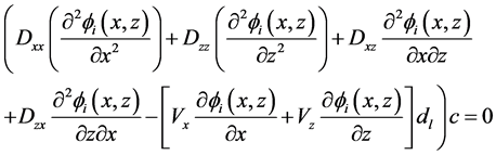
 (2)
(2)
where Dxx, Dzz, Dxz, and Dzx are dispersion tensor; c is the solute concentration; Vx and Vz are the seepage velocity in x and z directions.
Both these equations are coupled using the fundamental equation that relates fluid density, ρ to salt water concentration, c as follows:
 (3)
(3)
where ρ and ρf are contaminant fluid and freshwater density respectively. For the present study, some non- dimensional variables have been defined below as found in Rastogi et al. [8] as.
 (4)
(4)
 (5)
(5)
 (6)
(6)
where d is the depth of the confined coastal aquifer, V is the average linear velocity, c* is seawater concentration, αL and αT are the longitudinal and transverse dispersivities respectively. After replacing the above non dimensional variables in Equation (1) and (2) and after dropping primes in all terms for convenience, the following equations are obtained.
 (7)
(7)
where Kzz may vary from 0.0 to 1.0, and
 (8)
(8)
αT varies from 0.0 to 1.0 and the terms Dxx, Dzz, Dxz are defined in 2-D x-z coordinate system as suggested by Bear [21] ,
 (9)
(9)
 (10)
(10)
 (11)
(11)
Darcy’s equation for principal x and z axes can be written as
 (12)
(12)
 (13)
(13)
Equation (7), (8), (12), (13) constitute the governing equations for seawater intrusion in coastal aquifers. In Equation (8), Vx and Vz are defined as follows.
 (14)
(14)
 (15)
(15)
Here ; where
  (16)
(16)
θ is the porosity of the medium and 1/A is the head gradient of the fresh water. Dropping primes in all the above equation leads to
 (17)
(17)
Similarly
 (18)
(18)
 (19)
(19)
Dropping primes the above equation becomes
 (20)
(20)
Equation (17) and (20) give the velocity in non-dimensional form along the principal x and z directions respectively.
3. MFree PCM Formulation for Steady State Diffusive Interface Model
The MFree model is found to be an alternative numerical approach which eliminates the well-known drawbacks in finite difference, finite element and boundary element methods which accompany the grid based methods. In the present study, PCM based MFree model is developed and subsequently verified for the seawater intrusion problem in confined coastal aquifers based on a diffusive interface approach.
For discretizing the flow and transport equations, a PCM based meshfree strong form formulation proposed by Liu and Gu [22] is adopted. Initially a trial solution needs to be defined for  and
and  as [22]
 (21)
(21)
 (22)
(22)
where, hi is the unknown head at the ith node, and ci is the unknown concentration at the ith node. fi is the shape function which is again a function of  i.e. radial basis function (RBF) as given in Liu and Gu [22] and n is the total number of nodes in the support domain. Multi quadratics radial basis function (MQRBF) used presently is defined as:
 (23)
(23)
where, ; Cs and q are shape parameters of the radial basis function.
  where αc is the dimensionless size of support domain, and dc is the characteristic length that can be related to the nodal spacing in the local support domain. The value of shape parameter αc has a very profound impact on the accuracy of results. In the absence of an explicit method to find out the shape parameters, trial and error approach is adopted for its determination, which poses a certain limitation to the MQRBF method. The shape parameter q can be 0.5, 0.98 or 1.03 as suggested in Liu and Gu [22] . It is observed that standard Multi quadratic RBF has the q value of ± 0.5. In the present study the value of q is taken as 0.98 from Thomas et al. [15] . The derivatives of the unknown function at the collocation node xi can be expressed as
 (24)
(24)
For present study, the shape of the support domain is taken as circular where the radius can be varied according to accuracy required. Kovarik and Muzik [16] also used the concept of prescribing a radius for determining the supporting points. With a larger radius, more number of nodes will be present in the support domain but it will lead to an increase in the time of computation. Support domain can also be rectangular or square as adopted by Meenal and Eldho [13] . By implementing both Equation (21) and Equation (22) and also by using PCM, Equation (7) can be written as:
 (25)
(25)
where, ,
,  and
and  values are to be calculated for each support domain
which are subsequently incorporated in the global matrix for the whole problem domain with consideration of Kronecker delta property.
Further Equation (25) can be written in matrix form as:
 (26)
(26)
Similarly the transport Equation (8) can be approximated using PCM as
 (27)
(27)
Equation (27) can be simplified and written as,
 (28)
(28)
where [G2] and [G3] are global matrices of single derivative of fi with respect to x and z respectively [G4], [G5], [G6] and [G7] are global matrices of double derivative of fi with respect to x, z, xz, and zx respectively.
4. Model Development
Based on PCM based MFree formulation, a model in 2D was developed for diffusive interface seawater intrusion problem for a confined coastal aquifer in MATLAB. The specific steps in the modeling involve: 1) Discretization of the problem domain with nodes placed at a regular interval; 2) Specification of hydraulic conductivity, porosity, piezometric head gradient, depth of the aquifer, longitudinal and transverse dispersivity as input parameters; Variables are initialized and the initial head and concentration values are assigned; 3) Construction of support domain for all the nodes in the flow region. For every support domain single derivative of fi with respect to x and z and also double derivative of fi with respect to x, z, xz, and zx are found; 4) Assemblage of support domain matrix is assembled after applying boundary conditions into the global matrix; 5) Solution of the systems of equations for the state variables defining the head and solute concentration distribution in the flow domain. Initially for an assumed value of c, h is found which is used to compute c and the coupled equation is updated with the new c; 6) Progression of iterative solution till a user defined convergence is realized. Figure 1 shows the flowchart for the presently developed PCM based MFree model which was subsequently verified for its accuracy by examining its solution with two different well established research problems.
5. Case Studies
To investigate the effectiveness of the developed PCM model, the first case study considered is the well-recog- nized Henry’s problem [23] and the second work is a confined aquifer seawater intrusion problem reported by Pandit and Anand [3] .
5.1. Henry’s Problem
The domain of solution for this study is rectangular two-dimensional vertical cross-section of a confined coastal aquifer of length L and thickness d as shown schematically in Figure 2. The length-to-depth ratio for the problem domain is 2:1. The domain is bounded on top and bottom by impervious boundaries. A seawater body is there on right side of the problem domain and hence right boundary is referred as the seaward side and the left as landward side with freshwater inflow to the coastal aquifer.
The boundary conditions applied for the problem are relative concentration 0 at the fresh water inflow boundary and equal to 1 on the seaward boundary. Initial concentration in the aquifer domain is assumed to be 0. The mathematical representation of the applicable boundary conditions is listed in Table 1. A is the piezometric head gradient value substituted to take into account the inflow from the landward side which is taken as 151 to simulate the general inflow taken for the Henry’s problem.
To solve the Henry’s problem, after initial trials number of divisions considered in the x and z directions are 40 and 20 respectively. Consequently the number of nodes in the longitudinal and transverse direction is 41 and
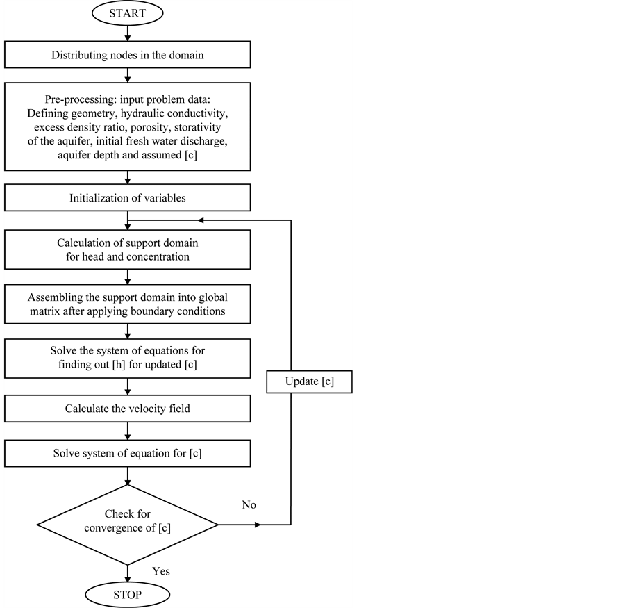
Figure 1. Flowchart for diffusive interface seawater intrusion model using PCM based MFree Method.
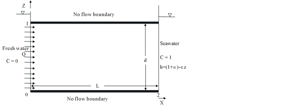
Figure 2. The geometry and boundary condition for the Henry’s problem.
21 respectively which makes the total number of nodes in the domain 861. The nodal distribution in the domain is as shown in Figure 3.
For the PCM model, q is presently considered as 0.98 adopted from Thomas et al. [15] after initial tuning of this parameter within a recommended range in literature varying from 0.5 to 1.03. Similarly αc is considered as 8 for both the case studies. A radial support domain was found appropriate with a radius equal to 3 times the nodal distance dc. For a dc value of 0.05, the radius of the support domain works out to 0.15. Figure 4 shows the solute mass concentration variation represented as isochlors for the Henry’s problem. The “S” shape of the isochlors indicates the existence of seawater circulation at the bottom of the aquifer and a reduction in the landward extent of seawater penetration due to dispersion as demonstrated by Henry [23] . In Figure 5, a comparison of 0.5 isochlor positions obtained by the present model with the solutions of [20] [24] [25] and [26] is presented.
The results obtained using the PCM model are in near alignment with the known solutions. A marginal shift in the position of 0.5 isochlor towards the landward side is noticed when compared to the existing solutions. The PCM produced shape of the interface is “S” type trending similar to the shapes given by other researches. The “S” shape of the interface suggests that in the top aquifer region, the intrusion is much less as when compared to the bottom of the aquifer. The shift of seawater wedge towards landward side is attributed to the assumed values of αT = 0.1 and dl = 0.8, (i.e. the velocity dependent dispersion effects) while other parameters are kept same. It is to be noted that previous models assumes dispersion coefficient to be independent of the velocity which is a concept lacking in simulation of real flow conditions. It can also be understood from the comparison that position of the toe (considering 0.5 isochlor as interface) is better predicted in the MFree method than by FEM as the proximity of the MFree solution is nearer to the semi analytical solutions [23] when compared to the FEM solutions. From the velocity vectors plotted in Figure 6, it is observed that there is a clockwise circulation of seawater in the zone of transition along the interface which has earlier been demonstrated by other researchers [3] [16] .

Table 1. Boundary conditions for the domain.
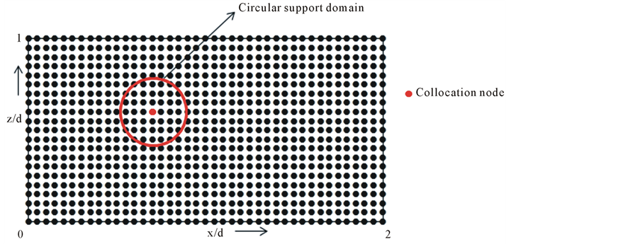
Figure 3. The nodal distribution for the Henry’s problem.
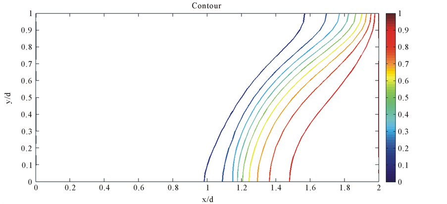
Figure 4. The solute mass concentration for the Henry’s problem.
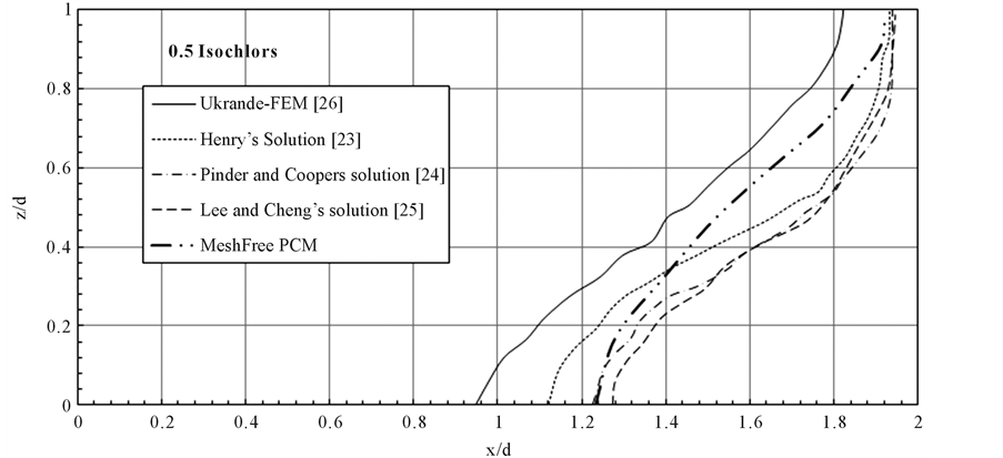
Figure 5. A comparison of the 0.5 isochlor for the Henry’s problem.
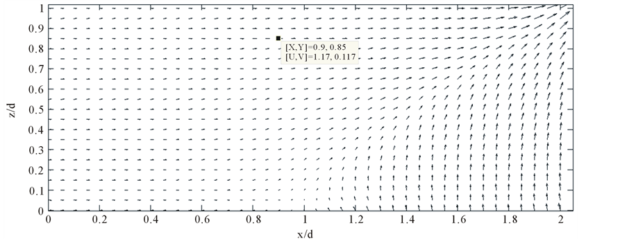
Figure 6. Velocity vector for the Henry’s problem.
5.1.1. Sensitivity Study of Meshfree Parameters
For the Henry’s problem, sensitivity of the model to number of nodes is performed to understand the effect of nodal distribution. The analysis is done by considering 210,861 and 3321 nodes in the domain. The 0.5 isochlors obtained for the Henry’s problem by varying the numbers of nodes 210, 861 and 3321 is shown in Figure 7.
It is encouraging that a larger nodal density involving 861 and 3321 nodes leads to near similar solutions. Presently simulation is performed on a Core i5 processor with speed of 3.1 GHz and 4 GB RAM. For a nodal specification of 210, 861 and 3321 nodes a computational time of 14.1322, 40.760, 248.944 seconds respectively was required for this configuration. This has suggested that after reaching a particular density of nodes in the domain, the accuracy of the result is not affected by increasing the number of nodes which is a positive outcome expected of a good numerical model. As expected when number of nodes is increased, the computational time also grows up considerably. It is thus understood from Figure 7 that increasing the number of nodes beyond certain limit does not improve the accuracy of the result further. This indicates a plausible strength of MFree simulation which is not much influenced by consideration of additional nodes in the flow domain and assumes a saving in simulation run time. FEM and FD solution scheme are known for nodal density dependence limiting their solution accuracy.
For the Henry’s problem, similar analysis was also carried out by varying the size of the support domain. Support domain is described as a function of number of times of the nodal distance. The simulation time required to model 861 nodal Henry’s problem for a support domain of 2 times the nodal distance was 33.03 seconds, where as three and four fold increase led to computational time increase to 40.76 seconds and 53.52 seconds respectively. The accuracy of the results however, remained almost the same in all the cases suggesting to keep the size of the support domain as minimum for the present problem without violating the Peclet number condition [22] . This analysis suggests robustness of the MFree simulation and recommends adopting a smaller support domain without sacrificing the accuracy of the solution.
5.2. Case Study 2
To further validate the applicability of the PCM model and to understand the pumping and recharge effects on seawater intrusion, a second case study from Pandit and Anand [3] for L/d ratio of 10:1 is considered. The rectangular two dimensional confined coastal aquifer with vertical cross section of length L and depth d is shown in Figure 8. The L/d ratio for the domain is 10:1 and data considered is as follows. A = 1000; KZZ = 1 porosity = 0.3, dl = 1.0 and αT = 0.1.
Relative concentration in the flow domain is 0 at the fresh water inflow boundary and 1 on the seaward boundary. Initial concentration in the aquifer domain is assumed 0. Boundary conditions for the problem are same as given in Table 1. For solving this problem, number of divisions considered after initial trials in the longitudinal x and transverse z directions were chosen 49 and 8 respectively. Consequently the number of nodes in x and z are 50 and 9 respectively. Thus the total number of nodes considered in the entire flow domain is 450. The nodal distribution in the problem domain is given in Figure 9. As stated earlier, the value of shape parameter q is considered as 0.98 and αc is taken equal to 8. Based upon the experience of earlier case study, a radial support domain was considered with a radius equal to 4 times the nodal distance. There is a fresh water flow from left to
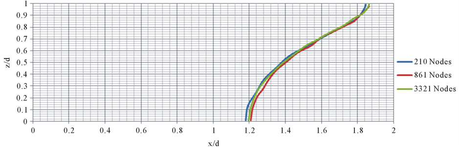
Figure 7. Comparison of 0.5 isochlors for different density of nodes.
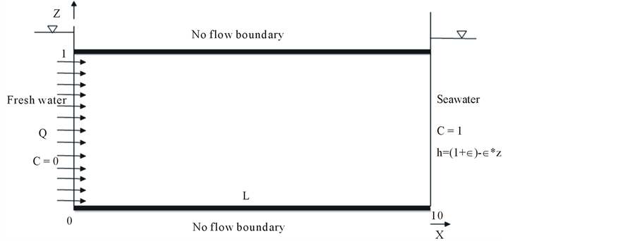
Figure 8. The geometry and boundary condition for Case study 2.
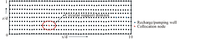
Figure 9. Nodal distribution of the aquifer.
right which is horizontal at the fresh water face. The piezometric head gradient in the study is expressed in terms of A and for the present problem is taken as 1000. The domain is bounded by no flow boundary condition on top and bottom. Figure 10 shows the solute mass concentration variation measured as isochlors. The 0.5 isochlors obtained in present model is compared with that of Pandit and Anand [3] and Ukrande [26] which are plotted in Figure 11. Comparison of 0.5 isochlors shows reasonable agreement. MeshFree results are closer to the Pandit and Anand [3] and validate the developed meshfree model.
Figure 12 shows the velocity vector for this case study. As seen in the figure, in the seaward side the hydraulic head gradient is found to be oriented vertically upward almost against the gravitational force points vertically downward. There is a fresh water inflow due to which solute density is less at the bottom portion of the domain. Velocity vectors also indicate the circulation of seawater inside the domain as shown in Figure 12.
6. Sensitivity Study of Parameters
Saltwater intrusion primarily depends on the four non dimensional parameters presently such as: A―Gradient of peizometric surface; αT―Transverse dispersivity; dl―depth of aquifer and Kzz―the ratio of principle hydraulic conductivity tensors. Here an attempt is made to study the influence of these parameters in the salt water intrusion using the developed PCM model. The ranges of the parameters studied are listed in Table 2.
6.1. Effect of Gradient of Peizometric Surface
The seawater intrusion to the costal aquifer depends on fresh water gradient or the inflow rate from the landward side to the seaward side. The gradient of the piezometric surface varies from 0.01% to 0.5% in most cases as observed by Pandit and Anand [3] . For present study, piezometric surface is expressed in terms of A as can be seen in Equation (16). The bound for the parameter Ais therefore established as 10,000 to 200. To understand the effect of piezometric head gradient on the intrusion process, plots of 0.5 isochlors were compared for dl = 1, Kzz = 1, αT = 0.5 while varying the values of A from 200 to 10,000. Figure 13 shows the variation of 0.5 isochlor for a set of chosen values of A. It was found from the study that with the larger values of A, the lesser is the piezometric head gradient at the landward side and hence the seawater encroaches further into the aquifer. It is found that this effect is more prominent at the bottom of the aquifer as observed in Figure 13.
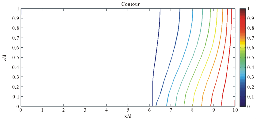
Figure 10. The distribution of solute mass concentration in the aquifer.
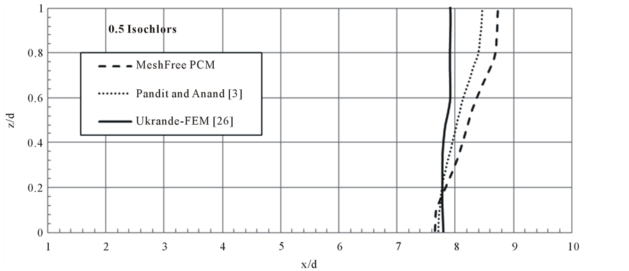
Figure 11. The spread of 0.5 isochlor (17,500 ppm) within the aquifer domain.
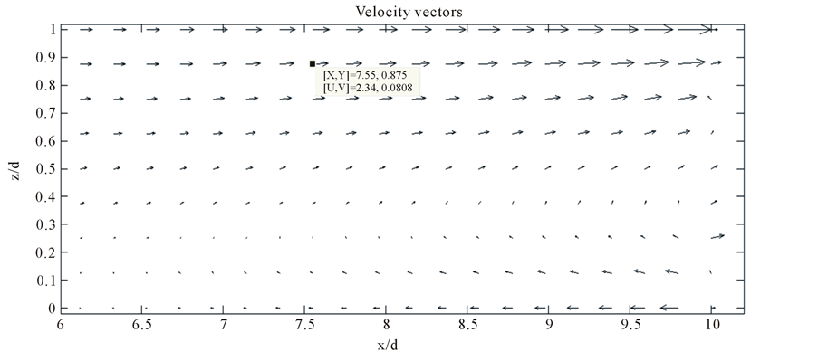
Figure 12. Velocity vectors for Case study 2.
Table 2. Range of field parameters.
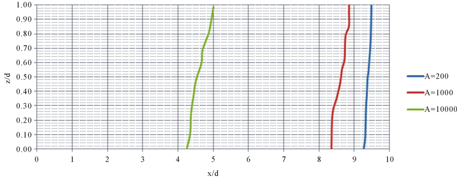
Figure 13. Variation of 0.5 isochlors for different piezometric gradient values.
6.2. Effect of Longitudinal Dispersivity and Transverse Dispersivity
The longitudinal dispersivity values are found much larger in the field than obtained in laboratory experiments. After compiling data inferred from various field tests Gelhar [27] recommended that longitudinal dispersivity would be in the range of tens of meters to few hundreds of meters. Here in order to consider the problem in the non-dimensional approach both longitudinal and transverse dispersivity is divided by longitudinal dipersivity as expressed in Equation (6). To study the effect of dispersivity, the range of αT which is presently the ratio of transverse to longitudinal dispersivity and therefore lower bound of 0.1 to an upper limit of 1.0 was adopted which is considered reasonable by Pandit and Anand [3] . Keeping the other parameters constant i.e. dl = 1, Kzz = 1, A = 1000, αT is varied from 0 to 1. Figure 14 shows the variation of 0.5 isochlor for the variation of αT. It was observed that with an increase in the value of αT, the seawater intrusion decreases as can be observed in Figure 14.
6.3. Effect of Depth of Aquifer
The depth of the aquifer is also another parameter that influences the encroachment of seawater into the fresh water. The depth of the aquifer normally varies in the range of 10 m to 500 m in the field problems. Here the non-dimensionalized parameter dl which is the ratio of aquifer depth to its longitudinal dispersivity as defined in Equation (6) is adopted for present sensitivity study. Larger aquifers generally have larger dispersivities and hence even though the depth of the aquifers varies from tens of meters to few hundreds of meters, a value ranging between 0.01 to 20 is found very reasonable for dl [3] . Figure 15 shows the 0.5 isochlors variation for different dl values. The study regarding the depth of the aquifer proved interesting as it was found that initially when the dl values are less, the 0.5 isochlors are found to be nearly vertical however with increase in the value of dl the isochlor tends to take more like S shape with more encroachment at the bottom of the aquifer as can be observed in Figure 15.
It is due to the fact that for higher values of dl the hydraulic effect causing cyclic flow becomes prominent as suggested by Cooper [28] whereas dispersion effects become negligible.
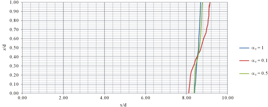
Figure 14. Variation of 0.5 isochlors for different αT values.
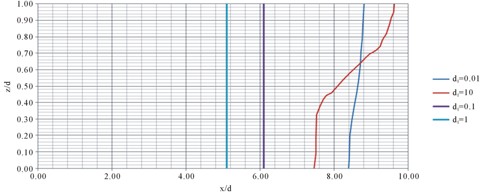
Figure 15. Variation of 0.5 isochlors for different dl values.
6.4. Effect of Hydraulic Conductivity
The property of hydraulic conductivity facilitates the movement of water through the porous media. The larger the pore size, the larger the hydraulic conductivity and vice versa generally holds true. To simplify the model, often a measured hydraulic conductivity value found by certain approach is used as uniform input value either for the entire model or for a particular grid. This method is suited for simulating the average response of the modeled system. In certain other approaches, spatial conductivity distributions from measured values are assigned to the model which is more tedious. The non-dimensional parameter Kzz is ratio of the hydraulic conductivity in transverse to the longitudinal direction as explained in Equation (5). It is commonly found that transverse hydraulic conductivity is lesser in magnitude than the longitudinal hydraulic conductivity. Presently, it is considered that Kzz vary from 0.1 to 1.0. To study the effect of anisotropy of the porous medium, all other parameter were kept constant and Kzz was assigned the values 0.1 and 1 in two respective cases. Figure 16 shows the 0.5 isochlor variation for different hydraulic conductivities. It was implicit that varying Kzz only produced a very small change in the location or shape of the isochlor as shown in Figure 16.
6.5. Effect of Pumping and Recharge
The flow equation formulated in the present study is for steady state and the time derivative term in the flow equation is taken as zero which assumes that release of water from the storage have negligible effect on the movement of seawater. To study the effect of pumping, well is simulated by applying a known head condition at the nodes corresponding to the depth of the penetration of the aquifers. Since pumping of ground water results in a decrease of aquifer head in the flow domain, to simulate steady abstraction well flow conditions, a marginally lower head is implemented on the well node than the surrounding area where well is installed. The equivalent discharge rate of the pumping well can be calculated with a standard discharge drawdown equation. Here two pumping wells are considered at location 125 m and 50 m respectively from the seaward side i.e. node 392 with x and y coordinates (8.75, 0.5) and another at node 428 (9.5, 0.5) as can been in Figure 9. At both these nodes, the imposed ratio of head on the well is 0.8 which is lesser than the surrounding area nodes. Figure 17 shows results with and without pumping effect for 0.5 isochlor. It can be observed from the Figure 17 that the 0.5 isochlor have moved towards landward side i.e. the toe of the 0.5 isochlor has shifted from 7.8 to 7.47 because of pumping of fresh water from these wells when compared to the isochlors of the domain without a pumping well.
Further the simulation is carried for recharge effects. The recharge wells cause an increase of groundwater head in the flow domain. To simulate a steady state recharge well, the head imposed on the well node is kept slightly higher than the nearby area nodes where it is installed. The equivalent recharge rate can be calculated from the relevant parameters of the well-known drawdown (or built up for this case) equation. Presently head ratio at node 218 (8.775, 0.5) is kept 1.2. Figure 18 shows the 0.5 isochlors with and without recharge effects. It can be seen from the Figure 18 that 0.5 isochlor has moved towards seaward side i.e. toe of the 0.5 isochlor is shifted from 7.8 to 9.4 because of injection of fresh water from these wells when compared to the isochlors of the domain without a recharge well.
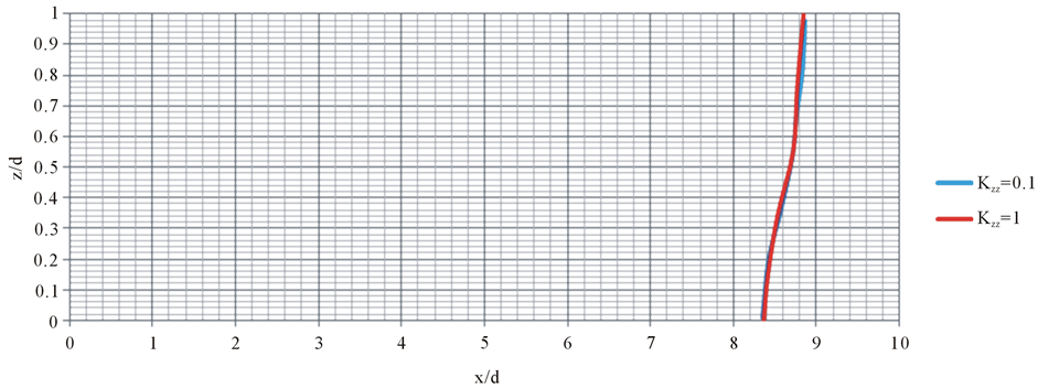
Figure 16. Variation of 0.5 isochlors for different ratios of principle hydraulic conductivity tensors.
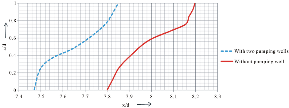
Figure 17. Comparison of 0.5 isochlors with and without pumping wells.
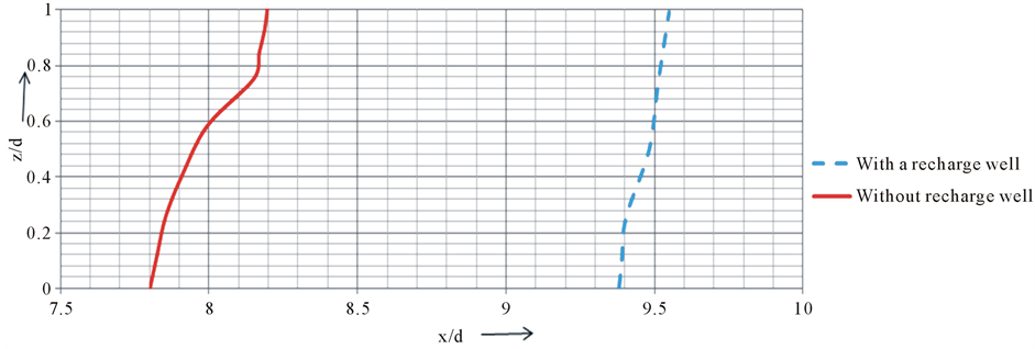
Figure 18. Comparison of 0.5 isochlors with and without recharge well.
It was also seen by the sensitivity analysis that the movement of the dispersive interface also depends on the location of the recharge or pumping wells. Location of pumping wells and well head was also found to play an important role in the sustainable freshwater yield from the costal aquifers. The advantage of this technique of well simulation is that the influence of well location and its penetration on the movement of interface can be adequately analyzed for practical considerations.
7. Concluding Remarks
In the present study, a simulation model based on PCM MFree method is developed for a confined coastal aquifer. The model is based on the diffusive interface approach using point collocation based MFree method. Adequacy of the model was established by comparing the results with well-known problems from the previous research works. Velocity vectors show the presence of circulation of seawater in the transition zone of the flow region. Further a sensitivity study of various parameters was carried out. The sensitivity study shows that a decreasing piezometric head gradient and increasing depth of the aquifer has more pronounced effect on the encroachment of seawater intrusion into the landward side when compared to the variation in the transverse dispersivity or the ratio of principle hydraulic conductivity tensors. An examination of the effects of injection and pumping wells revealed that proper control measures such as involving installation of recharge wells can be effectively used to seaward pushing of the salt-fresh water interface. Study suggests that location of wells can be an important determining factor in the movement of the dispersive interface and it is possible to analyze the interface push back effect for various locations of injection wells. Such simulation model can be coupled with optimization models to suggest optimal location of wells for adequate management of coastal aquifers. A comparison of the PCM model results with the available FEM model solutions showed that PCM results are marginally better when both (PCM and FEM) were compared with the available semi analytic concentration distributions. PCM based MFree model has advantages in preprocessing of meshing/remeshing and when appropriate PCM parameters are identified, the model is found to be computationally more effective. The proposed method may be a better choice for seawater intrusion studies in coastal aquifers.
Cite this paper
Alice Thomas,T. I. Eldho,A. K. Rastogi, (2016) Simulation of Seawater Intrusion in Coastal Confined Aquifer Using a Point Collocation Method Based Meshfree Model. Journal of Water Resource and Protection,08,534-549. doi: 10.4236/jwarp.2016.84045
References
- 1. Bear, J.A., Cheng, H.D., Sorek, S., Ouuzar, D. and Herrera, I. (Eds.) (1999) Seawater Intrusion in Coastal Aquifers— Concepts, Methods and Practices. Kluwer Academic Publishers, Dordrecht.
http://dx.doi.org/10.1007/978-94-017-2969-7 - 2. Rastogi, A.K. (2007) Numerical Groundwater Hydrology. Penram International Publication, India.
- 3. Pandit, A. and Anand, S.C. (1984) Groundwater Flow and Mass Transport by Finite Elements—A Parametric Study. In: Liable, J.B., Brebbia, C.A., Gray, W. and Pindereds, G., Eds., Proceedings of 5th International Conference on Finite Elements in Water Resources, Burlington, 363-381.
- 4. Bobba, A.G. (2002) Numerical Modelling of Salt-Water Intrusion Due to Human Activities and Sea-Level Change in the Godavari Delta, India. Hydrological Sciences Journal, 47, S67-S80.
http://dx.doi.org/10.1080/02626660209493023 - 5. Datta, B., Vennalakanti, H. and Dhar, A. (2009) Modeling and Control of Saltwater Intrusion in a Coastalaquifer of Andhra Pradesh, India. Journal of Hydro-Environment Research, 3, 148-158.
http://dx.doi.org/10.1016/j.jher.2009.09.002 - 6. Simpson, M.J. and Clement, T.P. (2003) Theoretical Analysis of the Worthiness of Henry and Elder Problems as Benchmarks of Density-Dependent Groundwater Flow Models. Advances in Water Resources, 26, 17-31.
http://dx.doi.org/10.1016/S0309-1708(02)00085-4 - 7. Qahman, K. and Larabi, A. (2006) Evaluation and Numerical Modeling of Seawater Intrusion in the Gaza Aquifer (Palestine). Hydrogeology Journal, 14, 713-728.
http://dx.doi.org/10.1007/s10040-005-003-2 - 8. Rastogi, A.K., Choi, G.W. and Ukarande, S.K. (2004) Diffused Interface Model to Prevent Ingress of Seawater in Multi-Layer Coastal Aquifers. Journal of Spatial Hydrology, 4, 1-31.
- 9. Li, J., Chen, Y. and Pepper, D. (2003) Radial Basis Function Method for 1-D and 2-D Groundwater Contaminant Transport Modeling. Computational Mechanics, 32, 10-15.
http://dx.doi.org/10.1007/s00466-003-0447-y - 10. Praveen Kumar, R. and Dodagoudar, G.R. (2008) Two-Dimensional Modelling of Contaminant Transport through Saturated Porous Media Using the Radial Point Interpolation Method (RPIM). Journal of Hydrogeology, 16, 1497-1505.
http://dx.doi.org/10.1007/s10040-008-0325-y - 11. Alhuri, Y., Ouazar, D. and Taik, A. (2011) Comparison between Local and Global Mesh-Free Methods for Ground-Water Modeling. International Journal of Computer Science Issues, 8, 337-342.
- 12. Meenal, M. and Eldho, T.I. (2011) Simulation of Groundwater Flow in Unconfined Aquifer Using Meshfree Point Collocation Method. Engineering Analysis with Boundary Elements, 35, 700-707.
http://dx.doi.org/10.1016/j.enganabound.2010.12.003 - 13. Meenal, M. and Eldho, T.I. (2012) Two-Dimensional Contaminant Transport Modeling Using Meshfree Point Collocation Method (PCM). Engineering Analysis with Boundary Elements, 36, 551-561.
http://dx.doi.org/10.1016/j.enganabound.2011.11.001 - 14. Swathi, B. and Eldho, T.I. (2014) Groundwater Flow Simulation in Unconfined Aquifers Using Meshless Local Petrov-Galerkin Method. Engineering Analysis with Boundary Elements, 48, 43-52.
http://dx.doi.org/10.1016/j.enganabound.2014.06.011 - 15. Thomas, A., Eldho, T.I. and Rastogi, A.K. (2014) A Comparative Study of a Point Collocation Based MeshFree and Finite Element Methods for Groundwater Flow Simulation. ISH Journal of Hydraulic Engineering, 20, 65-74.
- 16. Kovárík, K. and Muzík, J. (2013) A Meshless Solution for Two Dimensional Density-Driven Groundwater Flow. Engineering Analysis with Boundary Elements, 37, 187-196.
http://dx.doi.org/10.1016/j.enganabound.2012.10.005 - 17. Singh, L.G., Eldho, T.I. and Kumar, A.V. (2016) Coupled Groundwater Flow and Contaminant Transport Simulation in a Confined Aquifer Using Meshfree Radial Point Collocation Method (RPCM). Engineering Analysis with Boundary Elements, 66, 20-33.
http://dx.doi.org/10.1016/j.enganabound.2016.02.001 - 18. Kansa, E.J. (1990) Multiquadrics—A Scattered Data Approximation Scheme with Applications to Computational Fluid-Dynamics—II Solutions to Parabolic, Hyperbolic and Elliptic Partial Differential Equations. Computers and Mathematics with Applications, 19, 147-161.
http://dx.doi.org/10.1016/0898-1221(90)90271-K - 19. Contracta, D.N. and Srivastava, R. (1990) Simulation of Salt Water Intrusion in Northern Guam Lens Using a Microcomputer. Journal of Hydrology, 118, 87-106.
http://dx.doi.org/10.1016/0022-1694(90)90252-S - 20. Hamidi, M. and Yazdi, S.R.S. (2006) Numerical Modeling of Seawater Intrusion in Coastal Aquifer Using Finite Volume Unstructured Mesh Method. Proceedings of the 9th WSEAS International Conference on Applied Mathematics, Istanbul, 27-29 May 2006, 572-579.
- 21. Bear, J. (1979) Hydraulics of Groundwater. McGraw-Hill Publishing, New York.
- 22. Liu, G.R. and Gu, Y.T. (2005) An Introduction to Meshfree Methods and Their Programming. Springer, Dordrecht, Berlin, Heidelberg, New York.
- 23. Henry, H.R. (1964) Effect of Dispersion on Salt Encroachment in Coastal Aquifers. U.S. Geological Survey Water-Supply, Paper 1613-C, 70-84.
- 24. Pinder, G.F. and Cooper, H.H. (1970) A Numerical Technique for Calculating the Transient Position of the Saltwater Front. Water Resources Research, 6, 875-882.
http://dx.doi.org/10.1029/WR006i003p00875 - 25. Lee, C.-H. and Cheng, T.-S. (1974) On Seawater Encroachment in Coastal Aquifer. Water Resources Research, 10, 1039-1043.
- 26. Ukrande, S.K. (2003) Numerical Modeling of Multilayer Coastal Aquifers. PhD Dissertation, Department of Civil Engineering, IIT Bombay, Mumbai.
- 27. Gelhar, L.W. (1986) Stochastic Subsurface Hydrology from Theory to Applications. Water Resources Research, 22, 135S-145S.
http://dx.doi.org/10.1029/WR022i09Sp0135S - 28. Cooper, H.H. (1959) A Hypothesis Concerning the Dynamic Balance of Fresh Water and Saltwater in a Coastal Aquifer. Journal of Geophysical Research, 64, 461-467.
http://dx.doi.org/10.1029/JZ064i004p00461