Journal of Water Resource and Protection
Vol.06 No.06(2014), Article ID:45472,18 pages
10.4236/jwarp.2014.66062
Long Lead-Time Streamflow Forecasting Using Oceanic-Atmospheric Oscillation Indices
Niroj Kumar Shrestha
Department of Agriculture and Biological Engineering, University of Florida, Immokalee, USA
Email: nirojshrestha@ufl.edu
Copyright © 2014 by author and Scientific Research Publishing Inc.
This work is licensed under the Creative Commons Attribution International License (CC BY).
http://creativecommons.org/licenses/by/4.0/


Received 19 February 2014; revised 21 March 2014; accepted 15 April 2014
ABSTRACT
Climatic variability influences the hydrological cycle that subsequently affects the discharge in the stream. The variability in the climate can be represented by the ocean-atmospheric oscillations which provide the forecast opportunity for the streamflow. Prediction of future water availability accurately and reliably is a key step for successful water resource management in the arid regions. Four popular ocean-atmospheric indices were used in this study for annual streamflow volume prediction. They were Pacific Decadal Oscillation (PDO), El-Niño Southern Oscillation (ENSO), At- lantic Multidecadal Oscillation (AMO), and North Atlantic Oscillation (NAO). Multivariate Relev- ance Vector Machine (MVRVM), a data driven model based on Bayesian learning approach was used as a prediction model. The model was applied to four unimpaired stream gages in Utah that spatially covers the state from north to south. Different models were developed based on the com- binations of oscillation indices in the input. A total of 60 years (1950-2009) of data were used for the analysis. The model was trained on 50 years of data (1950-1999) and tested on 10 years of da- ta (2000-2009). The best combination of oscillation indices and the lead-time were identified for each gage which was used to develop the prediction model. The predicted flow had reasonable agreement with the actual annual flow volume. The sensitivity analysis shows that the PDO and ENSO have relatively stronger effect compared to other oscillation indices in Utah. The prediction results from the MVRVM were compared with the Support Vector Machine (SVM) and the Artificial Neural Network (ANN) where MVRVM performed relatively better.
Keywords:
Oscillation Indices, Streamflow, Lead-Time, Prediction

1. Introduction
The ocean-atmospheric indices are connected to climatic variability around the globe. Streamflow depends on the distribution of the precipitation in time and space as well as in the type and state of the basin, which, in turn, depends on the climatic conditions [1] . Annual streamflow volumes are more related to long-term climate therefore streamflow at this scale can be predicted using the long-term climate information. The teleconnection between climate and ocean/atmospheric oscillation indices is the scientific basis of long lead-time streamflow prediction.
Pacific Decadal Oscillation (PDO), El-Niño Southern Oscillation (ENSO), Atlantic Multi-decadal Oscillation (AMO), and North Atlantic Oscillation (NAO) are popular oceanic-atmospheric oscillation indices. The climate variation in the decadal-scale over the Pacific Ocean and its surrounding are strongly related to PDO which is coherent with the wintertime climate over North America [2] . ENSO has been linked to climate anomalies throughout the world [3] [4] . Strong ENSO signal exists in the mid-latitude United States that affects the flow in the river and streams [5] . Many prominent examples of regional multidecadal climate variability have been related to AMO. It affects air temperature and rainfall, and river flow over much of the Northern Hemisphere, in particular, North America and Europe [6] - [8] . NAO is a dominant mode of winter climate variability in the North Atlantic region ranging from central North America to Europe and much into the Northern Asia. There are several past studies for the long lead-time streamflow prediction using ocean-atmospheric oscillation indices. Streamflow responses to individual as well as coupled ocean-atmospheric modes of PDO, ENSO, AMO, and NAO over the United States are well established influencing signals [9] [10] . Chiew and McMahon [11] used ENSO-streamflow relationship to forecast streamflow successfully. Soukup et al. [12] predicted flows for North Platte River using PDO, ENSO, and AMO. Kalra and Ahmad [13] used these oscillation indices to predict long lead-time streamflow in the Colorado River basin.
The signal strength of oscillation indices varies spatially in the regions around the world. It is thus important to identify the influential oscillation indices or their combinations and corresponding lead time that develops the best prediction model for the given location of stream gages. Accurate prediction of long-lead time streamflow can benefit the management of water resources in the basin scale [14] . This is crucial information for water managers, stack-holders, farmers and others especially in the arid regions. Such prediction helps decision making process to maximize the returns from the available water resources and ensures reliable supply. Forecast with long-lead time also facilitates co-ordination between different system users that may be important in multiple-use water resource systems [9] .
There are several physically based models developed to understand the behavior of the water resources systems. The complexities in these models and difficulties associated with the data acquisitions and corresponding expenses that these models would require has limited the application of such models. To overcome these limita- tions, data driven models are often used as an alternative to physically based models. They are characterized by their ability to quickly capture the underlying physics of the system by relating inputs and outputs. They are robust and are capable of making reasonable predictions using historical data [15] [16] .
Artificial Neural Network (ANN), Support Vector Machine (SVM), and Relevance Vector Machine (RVM) are popular data driven models. The ANN model has ability to implicitly detect complex nonlinear relationship between response and predictors. It performs well even if the data contains noise. However, it has number of disadvantages. The ANN model may get stuck in local minima rather than global minima. Also, an incorrect network definition may cause over fitting of the model. The SVM model is a very popular machine learning model. It however makes unnecessary liberal use of the basis function. The number of support vector increases linearly with the size of training data [17] and the prediction is not probabilistic. Moreover, optimizing more than one model parameters in the SVM model needs cross validation. The RVM model is sparser than SVM and gives probabilistic output as well. Optimizing model parameter for the RVM model is relatively simpler, how- ever the performance is comparable. This study uses multivariate relevance vector machine (MVRVM) [18] model for predicting streamflow volumes which is an extension of the RVM algorithm developed by Tipping and Faul [19] .
The objective of this study is to identify the best combinations of oscillation indices and predict long-lead time annual streamflow volume accurately and reliably at four unimpaired stream gages in Utah that spatially covers the state from north to south.
2. Material and Methods
2.1. Study Area
Four stream gages were chosen in Utah (Figure 1). Each gage meets following data assumptions: 1) site flows are not affected by diversion or regulation, and 2) long year of systematic record is available. Two sites were chosen from northern Utah (Weber River near Oakley and Chalk Creek at Coalville) while each one from central (Muddy Creek near Emery ) and southern Utah (Sevier River at Hatch). The geometric characteristics of stream gages are shown in Table 1.

Figure 1. Location of the stream gages.

Table 1. Geometric characteristic of stream gages.
2.2. Relevance Vector Machine (RVM)
Relevance Vector Machine is a supervised learning model based on sparse Bayesian learning. This is a model of identical functional form to the SVM developed by Vapnik [20] [21] .
For the given input-target pair  in training data set, the model learns a dependency of the targets (streamflow in this study) on the inputs (oscillation indices) with the objective of making accurate predictions of the target (t) for previously unseen values of input x [17] [22] .
Target  is a sample from the model (
 ) with additive noise (
 ) which has mean zero with variance s2.
 (1)
(1)
The unknown function y is the product of design matrix (F) and weight parameter (w). In the vector form, Equation (1) can be written as,

where the target and weight vector are expressed as t = ( ……
…… )T and w= (
 ……
…… )T, respectively. An independent Gaussian noise is assumed. Thus,
  and the likelihood of complete da- taset is written as,
 (2)
(2)
To avoid the overfitting in Equation (2), w is constrained with prior probability (Equation (3)) [17] .
 (3)
(3)
where α is hyperparameter that controls the deviation of each weight from zero [23] . Bayes’ rule is used for ob- taining the posterior distribution over the weight.
 (4)
(4)
The posterior covariance and mean of the weight are  and
and  respectively, where
 .
.
For uniform hyperpriors over loga and logσ, .
.
 (5)
(5)
Equation (5) is solved by iterative re-estimation.
 and (6)
where . The term
  is the ith posterior mean weight and N is the number of data examples. The
  is the ith diagonal element of the posterior weight covariance computed with the current a and
 .
.
The learning algorithm proceeds by iterative process of Equation (6) together with updating the posterior sta- tistics  and
and  until some specified convergence criteria is satisfied. The predictions are made based on the posterior distribution over the weights, conditioned on the maximizing values
  and
and . The prediction for a new input (
 ) is given by,

where  and
and 
The model used in this study is one introduced by Thayananthan [18] . This is a Bayesian regression tool extension of the RVM algorithm developed by Tipping and Faul [19] . The Gaussian kernel was used in this study since it has shown to perform better than other kernels [23] [24] .
2.3. Data Collection
2.3.1. Streamflow
Unimpaired monthly streamflow data were collected for Weber River near Oakley, Chalk Creek at Coalville, Sevier River at Hatch, and Muddy Creek near Emery for 1950-2009 from the US Geological Survey (USGS). The values were then converted to annual flow volumes using appropriate conversion factor.
2.3.2. Pacific Decadal Oscillation (PDO)
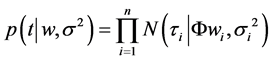
Pacific Decadal Oscillation (PDO) is a climate phenomenon associated with the persistent, bi-modal climate patterns in the North Pacific Ocean. It is an interannual climate index which can be used as an integrator of the overall winter climate conditions in the North Pacific. The PDO also refers to a numerical climate index based on the sea surface temperatures (SST) in a particular region of the North Pacific which has an interannual signature [25] . The pattern of PDO is similar to Pacific climate variability of ENSO however it has longer persistence. The PDO usually persist for 20 to 30 years. Both indices have similar spatial climate fingerprints but they have different behavior in time. Monthly PDO data were collected from the Joint Institute Study of Atmosphere and Ocean, University of Washington (www.jisao.washington.edu/pdo) and annual averages were computed for 1945-2009 (Figure 2(a)).
2.3.3. El-Niño Southern Oscillation (ENSO)
The El-Niño Southern Oscillation is a complex ocean/atmospheric interaction that causes cyclical patterns of warming and cooling of the sea surface in the tropical Pacific with the pronounced global climatic teleconnection. El-Niño is a warm-phase and La Niña is a cold phase. It has characteristic return frequency of 4 to 6 years, and usually persists for 1 to 2 years. Several studies have shown that it is associated with the streamflow variability in the western United States [10] . There are several ways ENSO can be represented. Southern Oscillation index (SOI) is one way to represent it [26] . It is computed from the monthly fluctuation in air pressure difference between Tahiti and Darwin, Australia. Positive values of the SOI are associated with the stronger Pacific trade winds and warmer SST. The monthly SOI values were collected from www.cdc.noaa.gov/ENSO/ for 1945-2009. Annual averages were computed from the monthly values for the entire analysis period (Figure 2(b)).
2.3.4. Atlantic Multi-Decadal Oscillation (AMO)
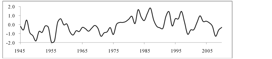
AMO index is introduced by Enfield et al. [6] as a simple basin average of North Atlantic Ocean (0˚ - 70˚) SST. It is a near-global scale mode of observed multi-decadal climate variability with alternating warm and cool phase over the large parts of the Northern Atlantic Ocean, with cool and warm phases that may last for 20 to 40 years at a time and difference of about 1˚F between extremes. Many prominent examples of regional mul- tidecadal climate variability have been related to AMO. The unsmoothened monthly AMO data were collected from www.cdc.noaa.gov/ClimateIndices/List/ . The annual average of AMO was computed for 1945-2009 (Fig- ure 2(c)).
2.3.5. North Atlantic Oscillation (NAO)
NAO is a dominant mode of winter climate variability in the North Atlantic region ranging from Central North America to Europe and much into Northern Asia. The positive NAO means below normal pressure across the high latitudes of the North Atlantic, and above normal pressure over the Central North Atlantic, Eastern United States and the Western Europe. This is opposite for the negative phase. The NAO index varies from year to year, but also exhibits a tendency to remain in one phase for intervals lasting for several years. The monthly average NAO data were collected from National Center for Atmospheric Research www.cgd.ucar.edu/cas/jhurrell/indices.html and annual averages were computed for 1945-2009 (Figure 2(d)).
2.4. Model Development
The input consists of annualized ocean-atmospheric oscillation indices and the output is the annualized streamflow volume. The oscillation indices at time step t were used to predict annual streamflow volume at time step t + i where  in years using the MVRVM. The data were divided into two parts: Training and Testing. The period 1950-1999 was used for training the model and the period 2000-2009 was used for testing. The model pa- rameter was optimized in the training phase and the performance of the model was evaluated based on RMSE,
 (a)
(a) (b)
(b)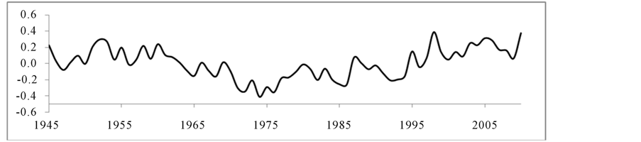 (c)
(c) (d)
(d)
Figure 2. Ocean Atmospheric Oscillation indices (a) PDO, (b) ENSO, (c) AMO, and (d) NAO.
correlation coefficient, and efficiency in the test phase.
Different models were developed based on the different combinations of oscillation modes in the input. Model 1 consists of using all four oscillation indices (PDO, ENSO, AMO, and NAO). This results in one model run for each lead-time. Model 2 consists of dropping one oscillation index and using remaining three oscillations. This results in four model runs for each lead-time. Model 3 consists of dropping two oscillation indices and using remaining pair. This results in total six model runs for a given lead-time. Model 4 consists of using only one oscillation mode at a time. This results four model runs for each lead-time. Model 1 is a base case while Model 2 to Model 4 gives the relative influence of ocean-atmospheric oscillation indices for the annual streamflow volume prediction for each selected gage. For each model type, the combination of oscillation indices and lead-time corresponding to the best test result was identified which was used to predict the long lead-time annual stream- flow volume. For each lead-time, the combination of oscillations that develops the best prediction was also identified. This shows the relative influence of oscillations for given lead-time for each selected gage. The prediction results from the MVRVM were also compared with the ANN and SVM.
3. Results and Discussion
3.1. Identification of Best Combination of Oscillation Indices and Corresponding Lead Time
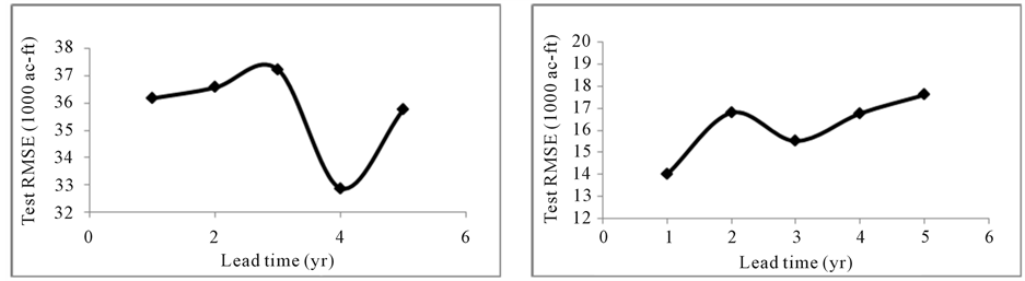
Model 1
Figure 3 shows the plot of test RMSE versus lead-time for annual streamflow volume prediction for Model 1. The smallest test RMSE was obtained at 4-year lead-time for Weber River near Oakley and Muddy Creek near Emery. This was, however, obtained at 1 year lead for Chalk Creek at Coalville. The second and third best test RMSE were obtained at 3 and 4 year lead, respectively. For Sevier River at Hatch, the test RMSE was relatively small at 3 and 5 year lead.
Model 2
Figure 4 shows test RMSE for Model 2 at 1 to 5 years lead for each gage. The smallest test RMSE was obtained at 4 year lead for Weber River near Oakley. This input corresponds to dropping NAO and using remaining three oscillation modes. Smallest test RMSE was obtained at 4 year lead for Chalk Creek at Coalville by dropping AMO. Dropping PDO at 4-year lead has similar test result. For Sevier River at Hatch, 3 year lead produced reasonable model prediction. This corresponds to dropping NAO and using remaining oscillation indices. The best test RMSE, however, was obtained at 2-year lead where the input corresponds to dropping AMO and using remaining indices. Comparable results were obtained by dropping PDO at 5-year lead. For Muddy Creek near Emery, 3- and 4-year lead produced relatively better results.
Model 3
The best test RMSE was obtained from the pair of PDO + ENSO at 4 year lead for Weber River near Oakley (Figure 5). The 3-year lead developed the best test RMSE for Chalk Creek at Coalville from ENSO + AMO pair, however comparable result was obtained at 4-year lead. For Sevier River at Hatch, a pair of PDO + NAO developed the best test RMSE at 2-year lead. PDO + NAO developed the best test RMSE at 2-year lead for Muddy Creek near Emery. Out of 6 combinations, 3 combinations resulted in poor prediction at 2-year lead. The test RMSE at 4-year lead was relatively better compared to 3- and 5-year lead which corresponds to ENSO + AMO.
 (a) (b)
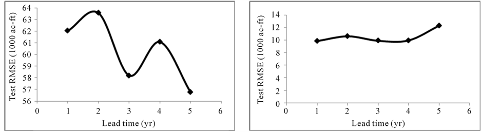 (c) (d)
Figure 3. Test RMSE for 1 to 5-year lead for annual streamflow prediction using Model 1 for (a) Weber River near Oakley, (b) Chalk Creek at Coalville, (c) Sevier River at Hatch, and (d) Muddy Creek near Emery.
 (a) (b)
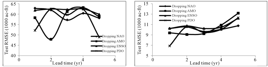 (c) (d)
Figure 4. The test RMSE at 1 to 5 year lead for annual streamflow prediction for Model 2 for (a) Weber River near Oakley, (b) Chalk Creek at Coalville, (c) Sevier River at Hatch , and (d) Muddy Creek near Emery.
 (a) (b)
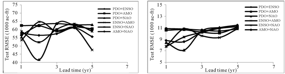 (c) (d)
Figure 5. The test RMSE at 1 to 5 year lead for annual streamflow prediction for Model 3 for (a) Weber River near Oakley, (b) Chalk Creek at Coalville, (c) Sevier River at Hatch, and (d) Muddy Creek near Emery.
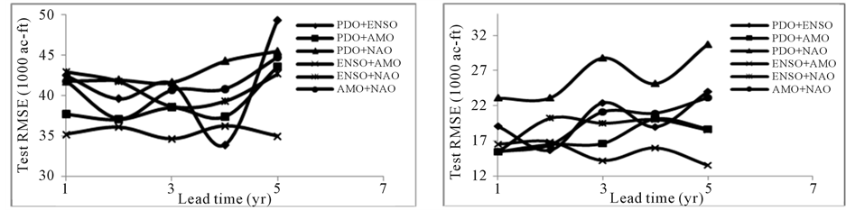
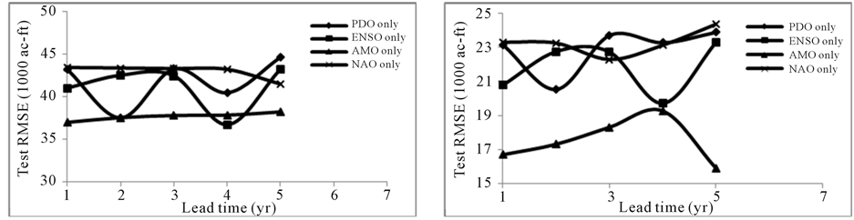
Model 4
The test RMSE at each selected gage for 1 to 5-year lead time is shown in Figure 6. ENSO developed the best model at 4-year lead for Weber River near Oakley. Comparable results were obtained from AMO at same lead
 (a) (b)
 (c) (d)
Figure 6. The test RMSE at 1 to 5-year lead for annual streamflow prediction for Model 4 for (a) Weber River near Oakley, (b) Chalk Creek at Coalville, (c) Sevier River at Hatch, and (d) Muddy Creek near Emery.
time. For Chalk Creek at Coalville, AMO produced relatively small test RMSE compared to other oscillation indices. However, the ENSO at 4-year lead developed the comparable model prediction. For Sevier River at Hatch, the PDO produced the best test RMSE at 2-year lead. Next to it, ENSO developed the best result at 4-year lead. For Muddy Creek near Emery, ENSO and PDO produced relatively better test RMSE at 1 and 2-year lead. When compared among 3-, 4- and 5-year lead, ENSO and AMO predicted relatively better at 4-year lead. In general, 4-year lead developed the best test result.
3.2. Prediction Results from Best Identified Combinations of Oscillations for Each Model
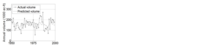
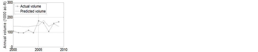
The best prediction for each model, the corresponding combination of oscillation indices, and lead-time for Model 1 to Model 4 are shown in Tables 2-5, respectively.
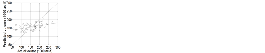
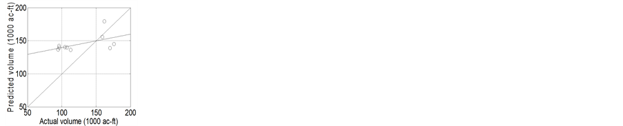
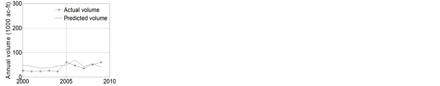
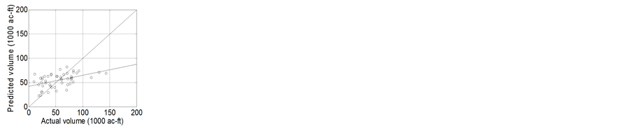
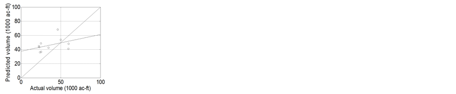
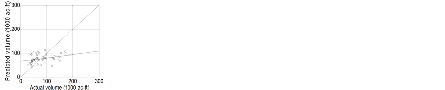
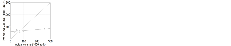
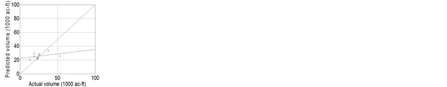
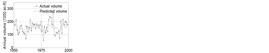
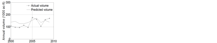
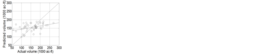
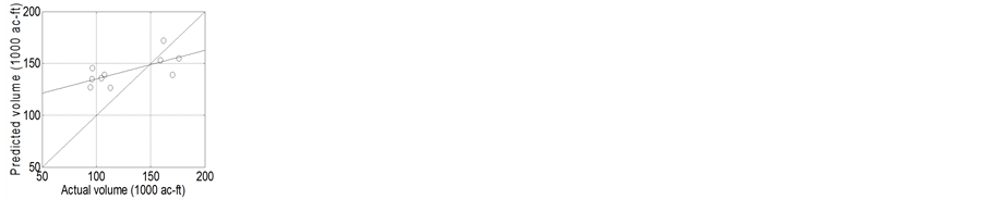
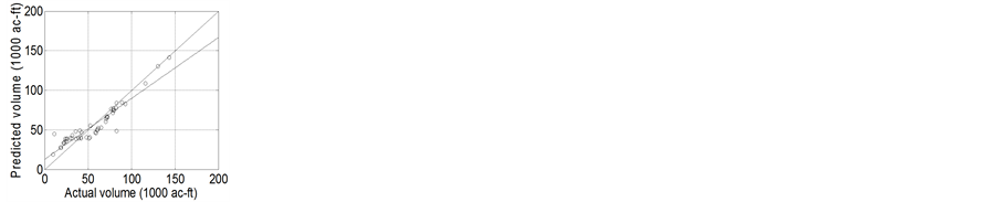
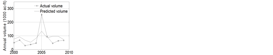
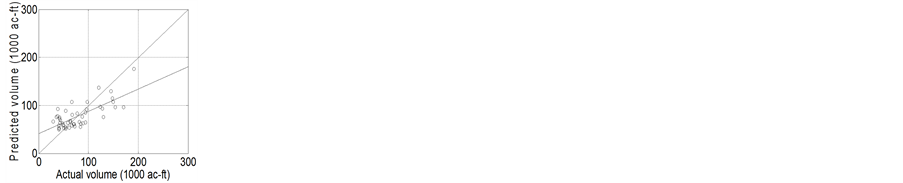
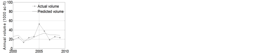
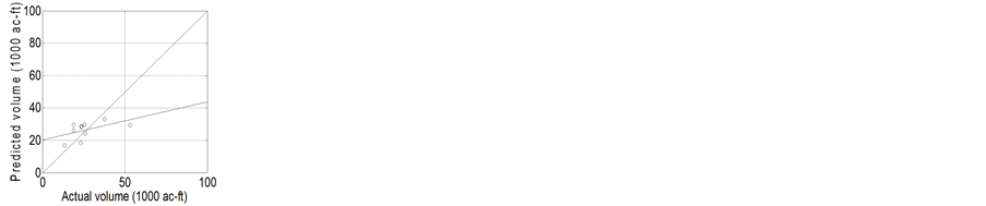
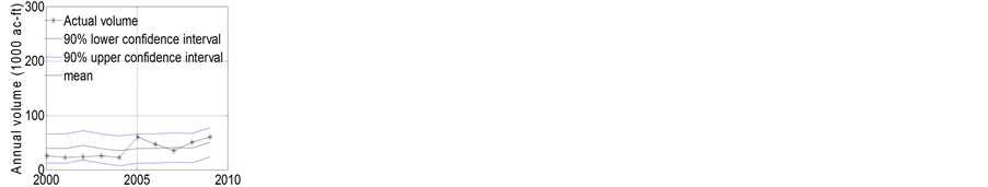
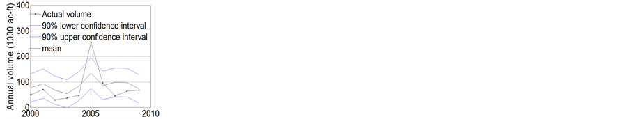
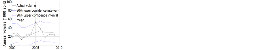
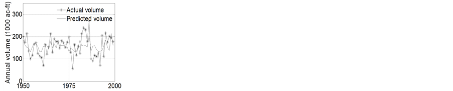
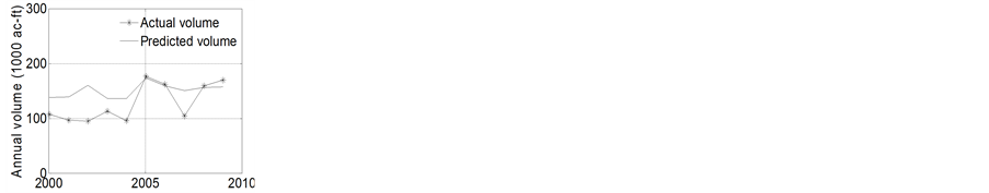
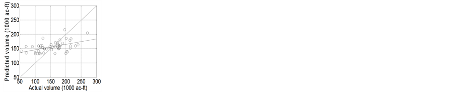
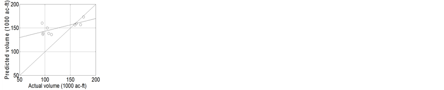
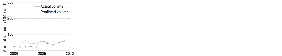
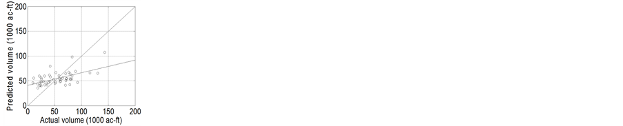
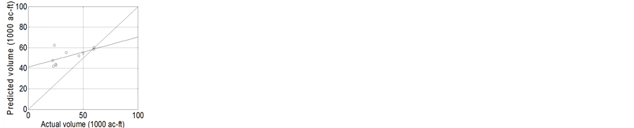
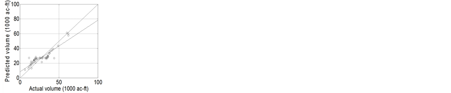
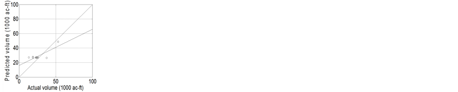
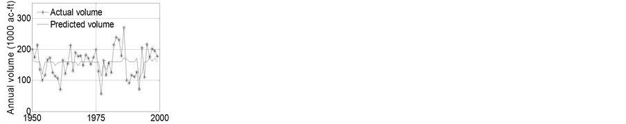
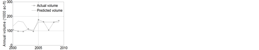
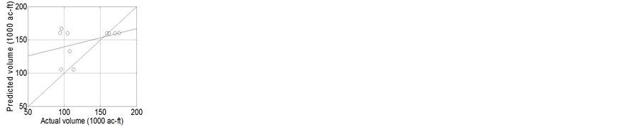
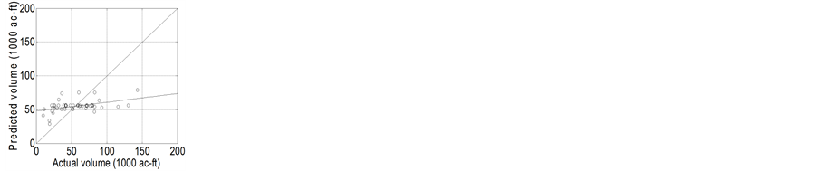
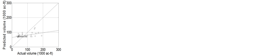
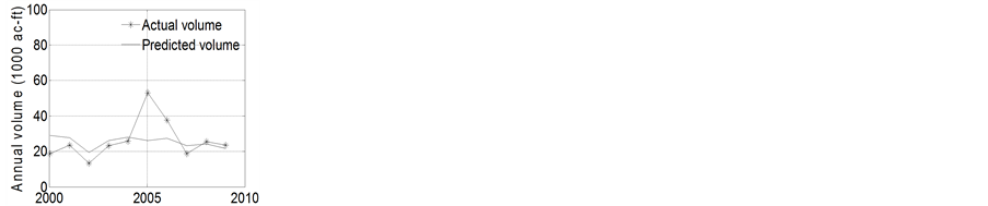
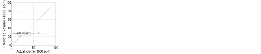
The predictions from Model 1 to Model 4 are presented in Figures 7-10, respectively. The first and second columns are for training and test phase, respectively. The third column is a plot of actual versus predicted annual flow volume for training phase and fourth column shows similar plot for the test phase. The results show that the model has predicted annual flow volume reasonably well using ocean-atmospheric oscillation indices. A good agreement was obtained between the actual and the predicted volume. The plot of predicted versus actual streamflow volume shows the points are saturated about 45 degree line except extreme flow events. This was because the oscillation indices do not fully represent the underlying physical processes responsible for generation of streamflow. In general, this prediction gives reasonable estimate of future water availability which could be used for planning and management of water resources in the basin scale.
3.3. Relative Strength of Oscillation Indices
Comparing Model 2 to Model 4 with the base case (Model 1), the relative influence of each oscillation index was estimated subjectively for each gage.
In Model 1, the best model prediction was obtained at 4-year lead for all stream gages except Sevier River at Hatch where the best model prediction was obtained at 3-year lead. Therefore, for comparing Model 2 (Figure 4) over Model 1 (Figure 3), 4-year lead was used for all stream gages except for Sevier River at Hatch where 3
Table 2. Prediction results, corresponding combination of oscillations and lead-time for Model 1.
Table 3. Prediction results, corresponding combination of oscillations and lead-time for Model 2.
*Second model.
Table 4. Prediction results, corresponding combination of oscillations and lead-time for Model 3.
Table 5. Prediction results, corresponding combination of oscillations and lead-time for Model 4.
*Second model.
year lead was used. Based on the test RMSE, the model prediction shows good improvement over Model 1 when NAO was dropped for Weber River near Oakley. Reasonable improvement was obtained when PDO was dropped. The model prediction marginally deteriorated when AMO was dropped. However, the prediction dete- riorated significantly when ENSO was dropped. For Chalk Creek at Coalville, significant improvement was ob- tained in the model prediction compared to Model 1 by dropping AMO, and PDO. Marginal improvement was obtained by dropping NAO, and ENSO. For Sevier River at Hatch, the prediction improved by dropping NAO. The result marginally deteriorated by dropping PDO and it deteriorated significantly by dropping ENSO. For Mud- dy Creek near Emery, the prediction results marginally deteriorated by dropping PDO, and NAO. It however
 (a)
(a)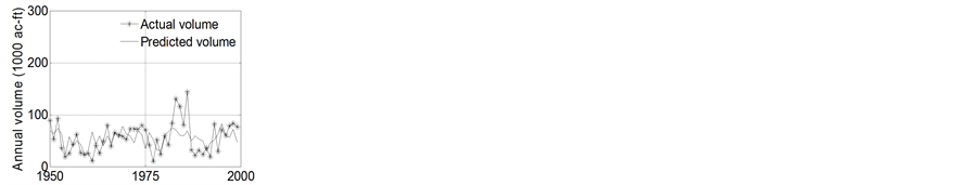
 (b)
(b)

 (c)
(c)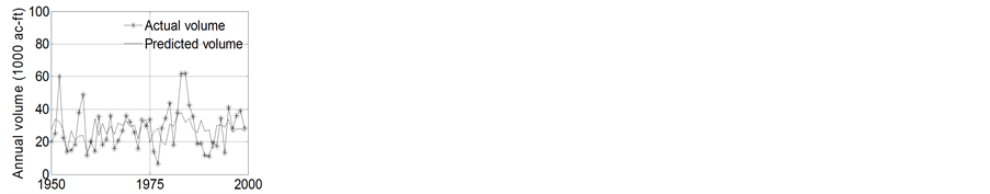


 (d)
(d)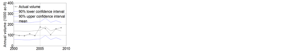
 (e)
(e)
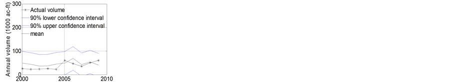
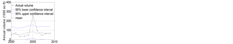
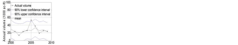
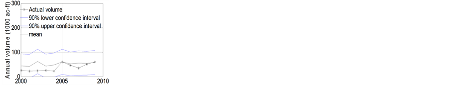
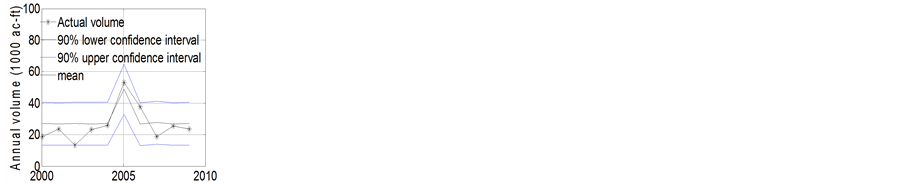
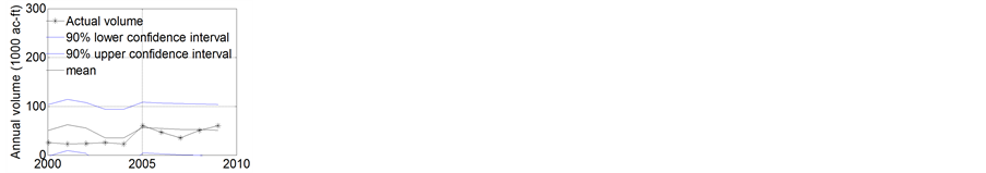
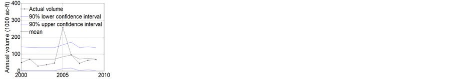
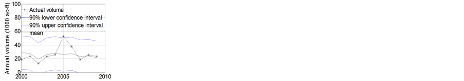
Figure 7. The plot of actual versus predicted annual flow volumes for Model 1 for (a) Weber River near Oakley, (b) Chalk Creek at Coalville, (c) Sevier River at Hatch, (d) Muddy Creek near Emery, and (e) 90% confidence interval of prediction in the test phase for all gages.
deteriorated significantly when ENSO and AMO were dropped. These comparisons help to identify the relative strength of the oscillation indices for each gage.
In learning machine, the model prediction deteriorates by the use of trivial predictors. Since the prediction re- sult improved by dropping NAO compared to Model 1 for Weber River near Oakley, NAO is not influential ocean-atmospheric oscillation index for annual streamflow volume prediction. The PDO and AMO have mar-
 (a)
(a)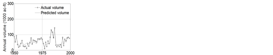

 (b)
(b)
 (c)
(c)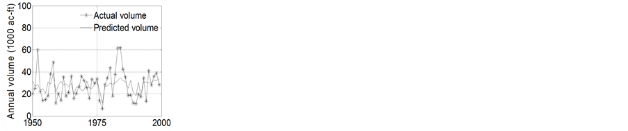

 (d)
(d)
 (e)
(e)
Figure 8. The plot of actual versus predicted annual flow volumes for Model 2 for (a) Weber River near Oakley, (b) Chalk Creek at Coalville, (c) Sevier River at Hatch, (d) Muddy Creek near Emery, and (e) 90% confidence interval of prediction in the test phase for all gages.
ginal influence while ENSO has strong influence because the prediction results significantly deteriorated com- pared to Model 1 when it was dropped.
For Chalk Creek at Coalville, AMO and PDO are not influential oscillation indices because the prediction re- sults improved compared to Model 1 when they were dropped. The ENSO and NAO, however has marginal in- fluence as prediction results marginally improved compared to Model 1 when they were dropped. NAO is not an
 (a)
(a)
 (b)
(b)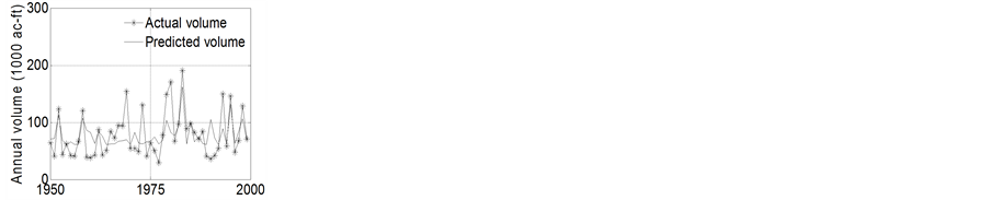


 (c)
(c)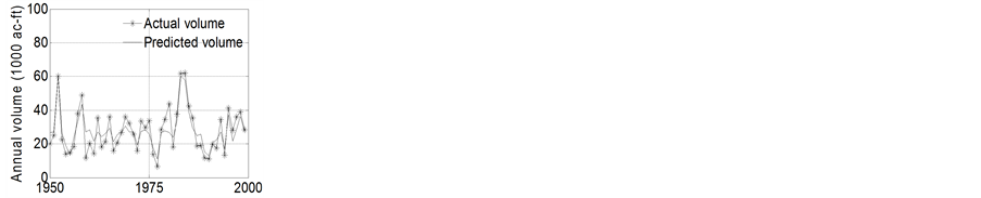

 (d)
(d)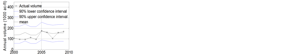

 (e)
(e)
Figure 9. The plot of actual versus predicted annual flow volumes for Model 3 for (a) Weber River near Oakley, (b) Chalk Creek at Coalville, (c) Sevier River at Hatch, (d) Muddy Creek near Emery, and (e) 90% confidence interval of prediction in the test phase for all gages.
influential oscillation index for Sevier River at Hatch because the prediction results improved when it was dropped. Since the results marginally deteriorated by dropping PDO, it may have marginal influence on the annual flow volume prediction. The prediction results however, deteriorated significantly by dropping ENSO. So, ENSO has strong signal for annual flow volume prediction for Sevier River at Hatch. For Muddy Creek near Emery, PDO and NAO have marginal influence and ENSO has strong influence for annual flow volume predictions.

 (a)
(a)

 (b)
(b)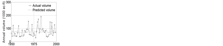

 (c)
(c)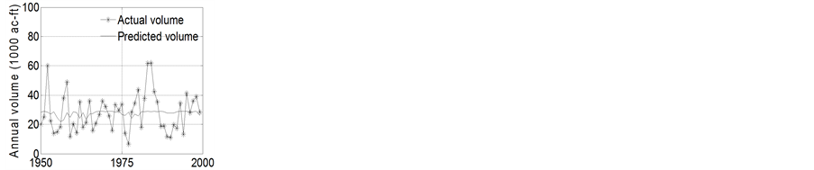
 (d)
(d)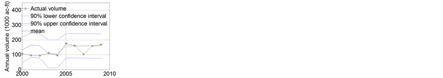
 (e)
(e)
Figure 10. The plot of actual versus predicted annual flow volumes for Model 4 for (a) Weber River near Oakley, (b) Chalk Creek at Coalville, (c) Sevier River at Hatch, (d) Muddy Creek near Emery, and (e) 90% confidence interval of prediction in test phase for all gages.
Based on the correlation coefficient between actual and predicted volume in the test phase, the overall results of Model 3 improved over Model 1. The relative strength of oscillation indices were again estimated subjective- ly by comparing results from Model 3 (Figure 5) to Model 1 (Figure 3). For Weber River near Oakley, the combination of PDO + ENSO developed similar model predictions as that of Model 1. Therefore, they may be considered as the influential ocean-atmospheric oscillation indices. The combination of PDO with NAO, and with AMO deteriorated the model prediction. The combination of ENSO with NAO, and with AMO also deteriorated the model prediction. This shows that the NAO and AMO do not have influential signal at Weber River near Oakley however, PDO and ENSO have strong influence. For Chalk Creek at Coalville, marginal improvement was obtained from ENSO + AMO pair over the base case. The prediction marginally deteriorated from the combination of PDO + ENSO. Other combinations significantly deteriorated the predictions. This shows that ENSO and PDO has marginal influence while other indices have week influence at Chalk Creek at Coalville. For Sevier River at Hatch, a pair of PDO + ENSO improved the model prediction compared to Model 1 while other pairs deteriorated the predictions. Some pairs marginally deteriorate the predictions while other pairs significantly. This indicates PDO and ENSO have relatively stronger signal at Sevier River at Hatch while other indices do not have influential effect. For Muddy Creek near Emery, combination of ENSO and AMO improved the model prediction.
Again, Model 4 (Figure 6) was compared with Model 1 and the relative effect of oscillation indices are discussed below. For Weber River near Oakley, the prediction from Model 4 did not improve but deteriorated compared to Model 1. However, the model predicted by ENSO was relatively better compared to other oscillation indices. Therefore, ENSO is likely to have relatively stronger signal than other oscillation modes for Weber River near Oakley. For Chalk Creek at Coalville, the prediction results did not improve compared to Model 1, however, ENSO, and AMO performed relatively better than other oscillation indices. This indicates ENSO and AMO have marginal influence while PDO and NAO have weak influence for Chalk Creek at Coalville. For Sevier River at Hatch, ENSO, and PDO marginally deteriorated the model predictions while AMO and NAO significantly deteriorated. This indicates ENSO and PDO have marginal influence while NAO and AMO do not have influential effect on Sevier River at Hatch. For Muddy Creek near Emery, ENSO and AMO perform marginally better than other oscillation modes. The ENSO and AMO thus have relatively influential signal while remaining two indices do not have influential signal for Muddy Creek near Emery.
In general, PDO and ENSO produced relatively better streamflow volume predictions compared to other annualized oceanic-atmospheric oscillation indices. The best model was usually obtained at 3 and 4 year leads. The best combination of oscillations can be used to develop accurate model prediction. In addition to fixing the lead time and identifying the best combinations of oscillation indices, the best combination of oscillations were also identified for each lead time (1 through 5 year) (Table 6) and were obtained from the different combinations of oscillation indices. This analysis shows that various combinations of oscillation indices can be used to en- hance the predictions for different lead-time. The ENSO and PDO, however, often predicted better than other oscillation indices for long lead-time annual streamflow volume.
3.4. Comparison with SVM and ANN
The results from the MVRVM for Model 1 to Model 4 were compared with corresponding SVM and ANN model for each gage. The software to develop SVM model was obtained from SVM and Kernel Methods Matlab Toolbox . The software to develop ANN model was obtained from Aston University Engineering and Applied Science (http://www1.aston.ac.uk/eas/research/groups/ncrg/resources/netlab/downloads/) . Figure 11 shows the comparison of MVRVM results with the SVM and ANN based on RMSE on test phase. For Weber River near Oakley, the MVRVM outperformed the ANN and SVM in Model 3 and Model 4 while the ANN and SVM performed relatively better in Model 1. For Model 2, MVRVM performed better than the ANN but slightly poor compared to the SVM. For Chalk Creek at Coalville, the MVRVM outperformed the ANN and SVM for Model 2 while the SVM outperformed others for Model 1. For rest of models, predictions from the MVRVM were better than the ANN, however, prediction results of the SVM and MVRVM were comparable. For Sevier River at Hatch, the MVRVM outperformed the ANN and SVM for all models (Model 1 - Model 4). For Muddy Creek near Emery, the prediction results among all three machine learning models were similar but the MVRVM performed relatively better than the ANN and SVM in all models (Model 1 - Model 4).
3.5. Bootstrap Analysis
A total of 500 bootstrap runs were used to construct the histograms. The 2.5th percentile and 97.5th percentile values of test RMSE were computed which are shown by red dotted lines in Figure 12. The narrow bound of histograms shows the model is robust. The test RMSE of actual model are in between two red dotted lines
Table 6. Best combination of oscillation indices for each lead-time.
 (a) (b)
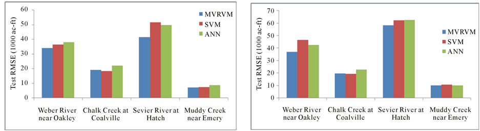 (c) (d)
Figure 11. Comparison test RMSE between the MVRVM, SVM, and ANN for (a) Model 1, (b) Model 2, (c) Model 3, and (d) Model 4.
indicating the developed model is robust and resonable to use as long lead-time streamflow prediction model.
4. Conclusions
The relationship between streamflow and climate variability represented by ocean-atmospheric oscillation indices is a key for the annual streamflow volume prediction. Accurate and reliable long-term streamflow prediction is crucial for the management of water resources in the basin scale. This study identifies the best combinations of the oscillations indices and lead-time for each selected stream gage and use them for the annual streamflow volume predictions. This study has also presented the relative influence of each oscillation index at each selected stream gage. The streamflow volumes were predicted at 1 to 5-year lead using the MVRVM model and pre- diction results were refined using the optimal combination of oscillations and corresponding lead-time. The model prediction showed satisfactorly results. Model 1 was a base case where all four oscillation indices (PDO, ENSO, AMO and NAO) were used while Model 2, 3, and 4 were developed from the different combinations of oscil- lation indices. The best predictions were usually obtained at 4-year lead-time. Although relatively better predic- tions were obtained at 2- and 3-year lead in some gages, the 4-year lead predictions were comparable. The ENSO and PDO generally predicted better than AMO and NAO for all gages. For the fixed lead-time used in this paper
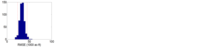

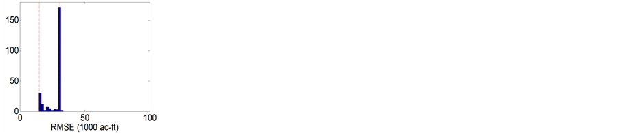
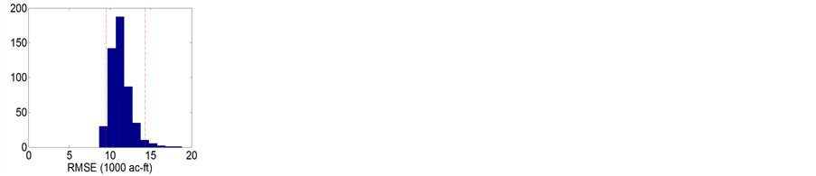


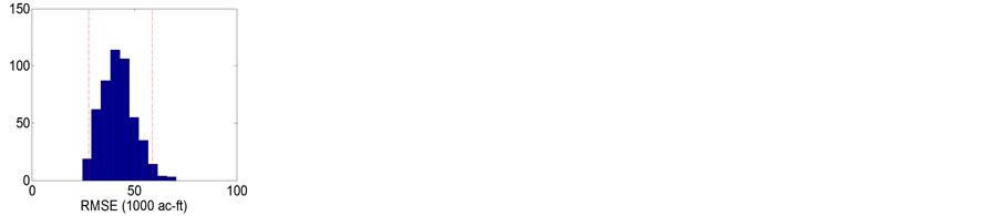
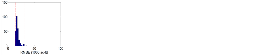
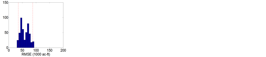


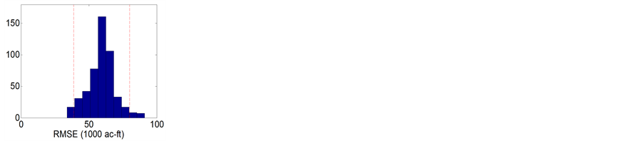
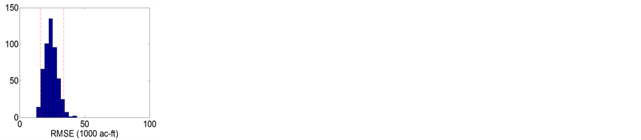
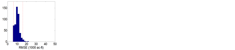
Figure 12. The bootstrap analysis for the best models. First column is for Weber River near Oakley, second is for Chalk Creek at Coalville, third is for Sevier River at Hatch, and the fourth is for Muddy Creek. Similarly the first row is for Model 1, the second is for Model 2, the third is for Model 3, and the fourth is for Model 4.
(4-year except Sevier River at Hatch), ENSO and PDO showed strong to marginal influence while AMO and NAO has weak to marginal influence. In addition, the combination of oscillations that predicted the best results for each lead-time were also identified. Different combinations of oscillations developed the best predictions at different lead-time. This information can be used to enhance the model predictions. In general, the model predicted reasonably well, however, it did not perform well on capturing the extreme events. This shows that the oscillation indices used in this paper are not enough to represent the physical process associated with the generation of streamflow. Bootstrap analysis was used to test the robustness and generalization capability of the model. The narrow bound of histogram showed that the model was robust. Also, the actual test statistics were in between the 2.5th and 97.5th percentile values which indicated the model prediction was consistent and was well generalized. The comparison showed that the MVRVM outperformed the ANN and SVM. The pattern of pre- dictions however remained similar in all machine learning models.
References
- Sivakumar, B. (2003) Forecasting Monthly Streamflow Dynamics in the Western United States: A Nonlinear Dynami- cal Approach. Environmental Modelling & Software, 18, 721-728.
- Mochizuki, T., Ishii, M., Kimoto, M., Chikamoto, Y., Watanabe, M., Nozawa, T., Sakamoto, T., Shiogama, H., Awaji, T., Sugiura, N., Toyoda, T., Yasunaka, S., Tatebe, H. and Mori, M. (2010) Pacific Decadal Oscillation Hindcasts Re- levant to Near-Term Climate Prediction. Proceedings of the National Academy of Sciences, 107, 1833-1837. http://dx.doi.org/10.1073/pnas.0906531107
- Diaz, H.F. and Markgraf, V. (2000) El Niño and the Southern Oscillation: Multiscale Variability and Global and Re- gional Impacts. Cambridge University Press, New York.
- Philander, S.G. (1990) El Niño, La Niña, and the Southern Oscillation. Academic Press, San Diego.
- Kahya, E. and Dracup, J.A. (1993) U.S. Streamflow Patterns in Relation to the El Niño/Southern Oscillation. Water Resources Research, 29, 2491-2503. http://dx.doi.org/10.1029/93WR00744
- Enfield, D.B., Mestas, N.A.M. and Trimble, P.J. (2001) The Atlantic Multidecadal Oscillation and Its Relation to Rainfall and River Flows in the Continental U.S. Geophyical Research Letters, 28, 2077-2080.
- McCabe, G., Palecki, M., Betancourt, J. and Fung, I. (2004) Pacific and Atlantic Ocean Influences on Multidecadal Drought Frequency in the United States. Proceedings of the National Academy of Sciences of the United States of America, 101, 4136-4141. http://dx.doi.org/10.1073/pnas.0306738101
- Sutton, R.T. and Hodson, D.L.R. (2005) Atlantic Ocean Forcing of North American and European Summer Climate. Science, 309, 115-118. http://dx.doi.org/10.1126/science.1109496
- Hamlet, A.F. and Lettenmaier, D.P. (1999) Columbia River Streamflow Forecasting Based on ENSO and PDO Climate Signals. Journal of Water Resources Planning and Management, 125, 333-341. http://dx.doi.org/10.1061/(ASCE)0733-9496(1999)125:6(333)
- Piechota, T.C., Dracup, J.A. and Fovell, R.G. (1997) Western US Streamflow and Atmospheric Circulation Patterns during El Niño-Southern Oscillation. Journal of Hydrology, 201, 249-271. http://dx.doi.org/10.1016/S0022-1694(97)00043-7
- Chiew, F.H.S. and McMahon, T.A. (2002) Global ENSO-Streamflow Teleconnection, Streamflow Forecasting and In- terannual Variability. Hydrological Sciences Journal, 47, 505-522. http://dx.doi.org/10.1080/02626660209492950
- Soukup, T.L., Aziz, O.A., Tootle, G.A., Piechota, T.C. and Wulff, S.S. (2009) Long Lead-Time Streamflow Forecast- ing of the North Platte River Incorporating Oceanic-Atmospheric Climate Variability. Journal of Hydrology, 368, 131- 142. http://dx.doi.org/10.1016/j.jhydrol.2008.11.047
- Kalra, A. and Ahmad, S. (2009) Using Oceanic-Atmospheric Oscillations for Long Lead Time Streamflow Forecasting. Water Resources Research, 45, W03413. http://dx.doi.org/10.1029/2008WR006855
- Asefa, T., Kemblowski, M., McKee, M. and Khalil, A. (2006) Multi-Time Scale Stream Flow Predictions: The Support Vector Machines Approach. Journal of Hydrology, 318, 7-16. http://dx.doi.org/10.1016/j.jhydrol.2005.06.001
- Khalil, A., McKee, M., Kemblowski, M. and Asefa, T. (2005) Sparse Bayesian Learning Machine for Real-Time Ma- nagement of Reservoir Releases. Water Resources Research, 41, W11401. http://dx.doi.org/10.1029/2004WR003891
- Khalil, A.F., McKee, M., Kemblowski, M., Asefa, T. and Bastidas, L. (2006) Multiobjective Analysis of Chaotic Dy- namic Systems with Sparse Learning Machines. Advances in Water Resources, 29, 72-88. http://dx.doi.org/10.1016/j.advwatres.2005.05.011
- Tipping, M. (2001) Sparse Bayesian Learning and the Relevance Vector Machine. Journal of Machine Learning Re- search, 1, 211-244.
- Thayananthan, A., Navaratnam, R., Stenger, B., Torr, P. and Cipolla, R. (2008) Pose Estimation and Tracking Using Multivariate Regression. Pattern Recognition Letters, 29, 1302-1310. http://dx.doi.org/10.1016/j.patrec.2008.02.004
- Tipping, M.E. and Faul, A.C. (2003) Fast Marginal Likelihood Maximization for Sparse Bayesian Models. Proceed- ings of the Ninth International Workshop on Artificial Intelligence and Statistics.
- Vapnik, V.N. (1995) The Nature of Statistical Learning Theory. Springer Verlag, New York. http://dx.doi.org/10.1007/978-1-4757-2440-0
- Vapnik, V.N. (1998) The Nature of Statistical Learning Theory. Springer Verlag, New York.
- Tipping, M. (2000) The Relevance Vector Machine. Proceedings of the Advances in Neural Information Processing Systems, The MIT Press, 652-658.
- Scholkopf, B. and Smola, A.J. (2002) Learning with Kernels: Support Vector Machines, Regularization, Optimization, and Beyond. MIT Press, Cambridge.
- Dibike, Y., Velickov, S., Solomatine, D. and Abbott, M. (2001) Model Induction with Support Vector Machines: In- troduction and Applications. Journal of Computing in Civil Engineering, 15, 208-216. http://dx.doi.org/10.1061/(ASCE)0887-3801(2001)15:3(208)
- Mantua, N.J. and Hare, S.R. (2002) The Pacific Decadal Oscillation. Journal of Oceanography, 58, 35-44. http://dx.doi.org/10.1023/A:1015820616384
- Poveda, G., Jaramillo, A., Gil, M.M., Quiceno, N. and Mantilla, R.I. (2001) Seasonally in ENSO-Related Precipitation, River Discharges, Soil Moisture, and Vegetation İndex in Colombia. Water Resources Research, 37, 2169-2178. http://dx.doi.org/10.1029/2000WR900395