Applied Mathematics
Vol.08 No.08(2017), Article ID:78834,16 pages
10.4236/am.2017.88090
An Optimal Cooling Schedule Using a Simulated Annealing Based Approach
Alex Kwaku Peprah1, Simon Kojo Appiah2*, Samuel Kwame Amponsah2
1Department of Computer Science, Catholic University College of Ghana, Sunyani, Ghana
2Department of Mathematics, College of Science, Kwame Nkrumah University of Science and Technology, Kumasi, Ghana

Copyright © 2017 by authors and Scientific Research Publishing Inc.
This work is licensed under the Creative Commons Attribution International License (CC BY 4.0).
http://creativecommons.org/licenses/by/4.0/


Received: September 2, 2016; Accepted: August 28, 2017; Published: August 31, 2017
ABSTRACT
Simulated annealing (SA) has been a very useful stochastic method for solving problems of multidimensional global optimization that ensures convergence to a global optimum. This paper proposes a variable cooling factor (VCF) model for simulated annealing schedule as a new cooling scheme to determine an optimal annealing algorithm called the Powell-simulated annealing (PSA) algorithm. The PSA algorithm is aimed at speeding up the annealing process and also finding the global minima of test functions of several variables without calculating their derivatives. It has been applied and compared with the SA algorithm and Nelder and Mead Simplex (NMS) methods on Rosenbrock valleys in 2 dimensions and multiminima functions in 3, 4 and 8 dimensions. The PSA algorithm proves to be more reliable and always able to find the optimum or a point very close to it with minimal number of iterations and computational time. The VCF compares favourably with the Lundy and Mees, linear, exponential and geometric cooling schemes based on their relative cooling rates. The PSA algorithm has also been programmed to run on android smartphone systems (ASS) that facilitates the computation of combinatorial optimization problems.
Keywords:
Simulated Annealing (SA), Variable Cooling Factor (VCF), Powell-Simulated Annealing (PSA), Global Minima, Rosenrock Functions, Android Smartphone Systems (ASS)

1. Introduction
Simulated annealing (SA) is a random search optimization technique that is very useful for solving global optimization problems involving several variables and ensures convergence to a global optimum [1] . It was inspired by the metallurgical process of heating up a solid and then cooling slowly until it crystallizes. The atoms of the heated solid material gain high energies at very high temperatures, giving them a great deal of freedom in their ability to restructure themselves. As the temperature is reduced, the energy of these atoms decreases until a state of minimum energy is achieved. However, if the cooling is not performed slowly enough, the process ceases to attain its minimal energy state [2] [3] [4] . Thus, an optimal cooling schedule, consisting of a set of parameters, needs to be designed to reach the required globally solution. For detailed discussions on SA, see Kirkpatrick et al. [2] , who originally proposed the method. Henderson, et al. [5] provides a comprehensive review of SA and practical guidelines for implementing cooling schedules while other readings can be found in van Laarhoven and Aarts [6] , Aarts and Korst [7] , Bryan et al. [8] , Tiwari and Cosman [9] and Thompson and Bilbro [10] . SA is a non-numerical algorithm which is simple and globally optimal, and well suited for solving the large-scale combinatorial optimization problems. Similar search algorithms such as the hill climbing, genetic algorithms, gradient decent, and Nelder and Mead Simplex (NMS) method are also suitable for solving optimization problems [11] [12] . SA’s strength is that it avoids getting trapped at either local optimum solution that is better than any other nearby. However, the SA algorithms still raise many open questions about the proper choice of cooling schedule (the process of decrementing temperature) parameters. For example, what is a sufficiently high initial temperature?; how fast should the temperature (cooling factor) be lowered?; how is thermal equilibrium detected?; and what is the freezing temperature? Among these questions, the most important and fundamental one is how to find a suitable cooling factor (β) that will help to reduce the computational time while getting a good optimum solution. Available literature on SA algorithms focuses mainly on the asymptotic convergence properties with less considerable work on the finite-time behaviour [5] . A careful search also indicates no known standard method for finding a suitable initial temperature and β-value for a whole range of optimization problems.
This paper seeks to propose a variable cooling factor model for SA schedule to speed up the annealing process. It further formulates the Powell-simulated annealing (PSA) algorithm [13] for finding global minima of functions of several variables. The PSA algorithm is then programmed to run on android smartphone systems (ASS) that facilitates the computation of optimization problems.
2. SA Cooling Schedule
2.1. Cooling Schemes
SA, as noted in the previous section, is a powerful search algorithm for solving global optimization problems. The rate at which the SA reaches its global minimum is determined by the cooling schedule parameters, which include the starting temperature, cooling factor, number of transitions at each temperature and other termination conditions [1] [14] . The most significant of these determinants (or parameters) is the cooling factor, which describes how SA reduces temperature to its next value. Numerous methods and algorithms have been used to determine the parameters of SA cooling schedule in various optimization problems. Kirkpatrick et al. [2] introduced the linear (or arithmetic) cooling schedule as given by Equation (1):
(1)
where is the new temperature value obtained from the old and is the amount of temperature reduction, kept constant and chosen from the interval [0.1, 0.2] while the initial temperature strongly depends on the problem being considered. van Laarhoven and Aarts [6] proposed the geometric cooling scheme described by the temperature-update scheme in Equation (2):
(2)
where and denote the new and old temperature values, respectively, and is the cooling factor assumed to be a fixed value in the interval [0.8, 0.99] [15] [16] . In another related study, Gong, Lin, and Qian [17] proposed the quadratic cooling schedule to estimate the number of iterations of the algorithm using a fixed value of selected from the interval (0, 1) . Nourani and Anderson [18] , using computer experiments, compared different proposed cooling schedules to find the cooling strategy with the least total entropy production at a given initial and final states and fixed number of iterations. Strenski and Kirkpatrick [19] compared two finite length cooling rates of linear and geometric schemes and found no significant difference in performance. They also concluded that high initial temperatures do not greatly improve the optimality of the algorithm when a geometric factor is used.
Lundy and Mees [20] argued that the stationary distributions for two succeeding values of the control parameter should be closed. This proposition is used to derive alternate decrement rules for selecting the cooling factor for SA cooling schedule. This proposition leads to the Lundy and Mees (L&M) model used to derive alternate decrement rules for selecting the cooling factor for SA cooling schedule, which is given by Equation (3):
(3)
where is a very small constant. Aarts and van Laarhoven [21] applied two different cooling rates, and 0.90, one after the other in a simple geometric cooling schedule for phase transitions of a substance. This approach allowed the SA algorithm to spend less time in the high temperature phases and more time in the low temperature phases thereby reducing the running time. Similar behaviour of SA was observed by Lin and Kernighan [22] in a SA algorithm for solving the travelling salesman problem (TSP).
2.2. Formulation of VCF Model
In this paper, we claim that the cooling factor should be a variable and not a fixed value as proposed by many authors hereinabove. A variable cooling factor (VCF) is a factor that decreases the temperature at each transition state during cooling process. Starting with a low value, the VCF increases gradually in value with number of transition states until the frozen point is reached. This section develops a variable cooling factor model that relates the cooling rates to transition states that a substance undergoes during the cooling process and size of a cost function. First, we consider the following theorems:
・ Theorem A:
If , the set of real numbers, where denotes non-negative real number, then and which follows that , the modulus of a sum of is not greater than the sum of the separate moduli [23] .
・ Theorem B:
Suppose and are continuous random variables with joint probability density function and let (ratio of the two random variables). Then has the probability density function [24] in Equation (4):
(4)
However, if and are independent, we obtain Equation (5):
(5)
Suppose are independent and identically distributed (iid) random particles of a substance that varies with temperature variations with standard deviation σ and mean number of particles μ. For simplicity, we let the random variables , for be independent standard normal random variables with marginal probability density function for each i be given by Equation (6):
(6)
Then the joint probability density function of the two independent random variables and is given by Equation (7):
(7)
Let us consider the transformation in Equation (8):
, (8)
which is a one-to-one transformation from to with inverses, and and the Jacobian,
(9)
Therefore, using the transformation technique (Theorem B), the joint probability density function of and is:
(10)
Using integration by parts, the probability density function of U is given by Equation (11):
(11)
which is the joint probability density function of random particles of the substance that varies with temperature variations. This joint distribution behaves as Cauchy distribution, which has flatter tails, making it is easier to escape from local minima. Now if we let assumes a Cauchy distribution, μ be any real number and σ > 0, then [25] [26] . Then Equation (11) can be re-written using the real-valued parameters μ and σ as;
(12)
where σ and μ are the standard deviation and mean, respectively. From Equation (12), we let
(13)
Then by using Equation (13) and Theorem A, we have Equation (14):
(14)
Let the number of variables (size) of the cost function be v, where . Then putting
, (15)
where is the total number of iterations in the system, we obtain the Equation (16):
(16)
for ; the number of cycle counts in the system; and , the fixed number of iterations in each transition state before the temperature is updated. That is, for , the square of deviations are inversely proportional to the square root of sum of the number of variables in the cost function and number of iterations at each transition [27] . Now combining Equations (14) and (16) yields Equation (17):
, (17)
which is the rule by which the random particles of a substance loose energy to the surroundings. Hence, the new cooling scheme for the annealing process is given by Equation (17) and the temperature-update formula is by Equation (18):
(18)
where is the variable cooling factor, which depends on the number of transition states k.
2.3. Test of VCF Model
A simulated annealing cooling scheme that is relatively slow has the ability to avoid premature convergence of local minima and thus provides good solution of optimization problem. The VCF model as developed in Equation (17) will be tested for this property against the various known cooling schemes in literature. Three of these cooling schemes, namely, Lundy and Mees (L & M), geometric and linear (or arithmetic) as represented by Equations (19), (20) and (21), respectively, were chosen and compared their relative cooling rates with the VCF in Equation (17):
(19)
(20)
(21)
where the parameter n is the number of iterations in each transition state In each of the three cooling schemes in Equations (19)-(21), the temperature is updated at each iteration. Hence, for each temperature and the parameters and are the fixed cooling factors associated with the Lundy and Mess, geometric and linear cooling schemes, respectively. Three main settings were made by putting and number of iterations = 25 and applied to Equations (17), (19)-(21). The temperature declination of each cooling scheme is obtained as illustrated in Figure 1.
From the settings, the values of cooling factors selected for L&M, geometric, and linear cooling schemes were , and , respectively and kept constant, whilst that for VCF was varied gradually from 0.875 to 0.890 during the cooling process.
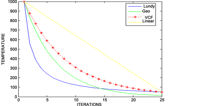
Figure 1. Temperature decline by the linear, geometric, Lundy and Mees (L&M) and VCF cooling schemes.
As it can be seen from Figure 1, during the first 15 iterations, L&M and geometric cooling curves decline faster in the initial high temperatures than the VCF and linear cooling curves. Between iterations 14 and 25, the cooling curves of the L&M and geometric slow down more gently to the minimum temperature, with the geometric having better cooling rate than the L&M and linear. However, the temperature declination of VCF curve is found to be gentle and smooth right
from the initial temperatures to the minimum temperature. Its rate of cooling is more preferred to the other three cooling schedules, which presupposes that the VCF will fit well into the SA algorithm.
3. SA Algorithm and Powell’s Method
As indicated in Section 1, SA is a random search optimization technique that is very useful for solving global optimization problems involving several variables without calculating derivatives and also ensures convergence to a global optimum [1] . One advantage of SA algorithm is that it is able to avoid getting trapped at local solutions while the principal drawback of SA is its intensive computational time requirements. The Powell’s algorithm, however, is a method used to search for minima of n-dimensional quadratic functions whose partial derivatives are assumed to be unavailable. This method depends on the properties of conjugate directions, denoted by quadratic functions and linearly independent directions, being columns of unity identity matrix. It converges to the required solutions in transitions. The drawback of the Powell’s method is that, for non-quadratic problems, as the algorithm progresses, the “conjugacy” of the direction vectors tend to deteriorate, making the algorithm difficult to converge to the required solution.
In this study some steps of the Powell’s method will be modified and combined with the simulated annealing algorithm to produce a new algorithm as presented in the next section. It is expected that the new algorithm can be used to search for global solutions of combinatorial optimization problems in a very good time.
The SA algorithm and Powell’s method are summarized and presented in Table 1.

Table 1. The SA algorithm and Powell’s method.
4. PSA Algorithm for Global Minimum
Some of the parameters of the Powell’s algorithm were modified and incorporated into the annealing algorithm to form a new SA algorithm called Powell-simulated annealing (PSA) algorithm. These parameters included the direction vectors, initial guess, and cycle count techniques. The proposed PSA algorithm template for finding global minimum of function of several variables is presented below.
PSA ALGORITHM:
Step 1:
a) Select a starting point (in N dimensions) and calculate [need stopping criteria].
Set .
b) Choose a random point on the surface of a unit N-dimensional hyper- sphere to establish a search direction, S.
c) Select an initial temperature T > 0
Step 2:
While T > lower bound, do the following:
a) Minimize f in each of N-normalized search directions. The function value at and at each search is . Note:
b) Compute ;
c) If (downhill move); Set
d) If (uphill move); Set with probability,
Step 3:
a) Compute the average direction vector and minimize f in the direction
Set
b) Set (reduce temperature by cooling factor ) and go to step (4).
Step 4:
Repeat steps 2 and 3 until the algorithm converges.
The steps 3 and 4 of the Powell’s method were not included in the PSA algorithm. The detailed description of PSA algorithm is presented under the implementation in Section 4.2.
4.1. Move Generation Model
The move generation model for minimizing function of single variable problems is presented. Let the new solution and , then compute the α-value using the formula in Equation (22):
(22)
where is the initial solution; is the neighbourhood of the current solution ; are the transition states, and the current solution where and a and b are the lower and upper of the domain, respectively. Thus, in our SA algorithm, instead of selecting a random number, α-value from tables, we estimate it using Equation (22). The random move generation strategy in the SA algorithm is replaced by the α-model in the proposed PSA algorithm.
4.2. Implementation of PSA Algorithm
The PSA algorithm is aimed at searching for global minimum of multi-dimensional functions in combinatorial optimization problems. The proposed PSA algorithm is implemented via the VCF model to speed up the annealing process and also to find the global minima of given cost functions of several variables. The cost function is defined over an N-dimensional continuous variable space, where
(23)
The problem is how to use the PSA to find the global minimize , satisfying the condition in Equation (24), called the global minima.
(24)
A detailed implementation of the PSA algorithm for finding global minimize followed by the following steps:
Step 1:
The initial data (or parameters) of the function and PSA are stated together with the floating point representation of the data, . A random starting point (domain) is selected and computed. The domain is defined by . The is a rectangular subdomain of , centered at the origin and whose width, along each coordinate direction is determined by the corresponding component of the vector a. The value of is checked to be feasible or exits within the tolerance level of (stopping criterion). This is repeated several times till the feasible value of is obtained. Set to be linearly independent coordinate directions (in n-dimensions) and assume that the directions are normalized to unit length so that where denotes the Euclidean norm. The initial temperature together with the temperature decrement formula, are stated, where .
Step 2:
In each (transition states k), where , starting from the point , a random point is generated along a given n-normalized direction vectors, from S such that
(25)
where is the component of the step vector along the coordinate direction. Equation (25) is then used to transform or reduce to a single variable problem as:
(26)
Equation (22), also known as the golden search method, can be applied to calculate the value of to minimize Equation (26) along the n-unidirectional search directions. That is, at each iteration, the factor is used to perturb the present configuration into a new configuration such that:
(27)
The probability that the current solution will be accepted or rejected is given by the Metropolis criterion:
(28),
where . If , then and is accepted, return to Step 3.
Else, compute and generate a random number . If , then the iteration step is accepted and the next direction vector in the cycle is selected. Else, no change is made to the vector. Go to Step 1.
Step 3:
This step completes the iterations in a transition by computing the average direction vector , normalized to and determined as before to minimize . The current solution is set to and the temperature is updated using . This completes the iterations in the first transition state and number of iterations at this state is given by .
Step 4:
Steps 2 and 3 are repeated until the algorithm converges to the global solution (minimum).
Unlike the Powell’s iterations, the direction vectors are not replaced one after the other, in this case. The worse solutions or vectors are accepted or rejected based on the Metropolis criterion (Step 2). The normalized average direction vector is computed to preserve the linear independence of the directions vectors at each iteration and termination of a transition.
To examine the performance of the PSA algorithm, it was tested against the NMS method and SA algorithm with the geometric cooling scheme. The proposed test functions included the Rosenrock functions of 2 dimensions in Equation (29), the Powell quartic function of 4-D in Equation (30) and other multi-minima functions of N dimensions in Equation (31):
(29)
(30)
(31)
These methods have been reported to be simple, reliable, and efficient global optimizers [12] [29] . They are sometimes able to follow the gross behaviour of the test functions, despite their many local minima. The selected test functions are among the classical NP-complete combinatorial optimization problems and are indeed a hard test for every minimization algorithm. The PSA method was tested on the Rosenbrock functions in 2-D followed by Powell quartic function in 4-D. The admissible domain of the 2-D function was (−200, 200) and Powell’s quartic function was used on (−50, 50). The PSA algorithm and the other methods it is being compared with were started from the same points randomly chosen from the domains, quite far from the origin. The starting temperature of each test was chosen by the design to be in the range 60˚C - 240˚C. The β- value in the PSA algorithm was made to vary while in the other algorithms, the β- value was kept fixed. The PSA web program was used to run each test 20 times and the best solution in each case recorded as shown in Tables 2-4, respectively in Section 5.
4.3. PSA Android Mobile Application
The SA algorithm is, so far, commonly available in FORTRAN, PASCAL, MATLAB, C and C++ programs. This makes the SA algorithm inaccessible by most of the mobile phones due to the incompatible operating systems. One achievement of this work is the development of an optimal SA cooling schedule model which can portably be programmed to make running of the SA algorithm on android smartphone systems possible. The running proceeds as follows:
・ Accessing PSA on Android Platform and Internet:
There are two options to access the App, by mobile application and Web access. The mobile application will download and install the application (Scudd PSA) from Google Play Store while the Web access follows the link: http://www.scudd-psa.byethost7.com.
・ Running PSA Pseudo Code on ASS:
Given the optimization problem in Equation (32):
(32)
(i) Input the parameters: and .
(ii) Press the run key for the output (results).
5. Test Results and Analysis
5.1. PSA Accounting for Cooling Schemes
The first test was performed using six different cooling schemes one after the other on the Rosenbrock function in 2 dimensions (Equation (29)) to find the computational time of the PSA algorithm. The standard cooling factors of the five search schemes were selected for the test while the VCF was made to vary gradually from 0.875 to 0.890. The schemes were all started from the same point (24, 20), randomly chosen from the domain. Each test was run 25 times over the interval [−200, 200]. The mean optimal results obtained for the six test schemes are reported in the Table 2.
In the 2 dimensions with a tolerance level of , the geometric, exponential and VCF schemes slightly deviated from the global minimum at the origin (see Table 2). The average distance from the optimal value was found to be 1.00E−05, 1.33E−05 and 1.00E−05 for the geometric, exponential and VCF schemes, respectively. The cost of running each scheme was estimated in terms of the total number of transitions per second. This was very high for the geometric with 20 transitions in 1.300 seconds, low for exponential scheme with 5 transitions in 0.910 second and lower in VCF with 3 transitions in 0.600 second.
Table 2. Comparison of mean optimal parameters’ values of the six cooling schemes on Rosenbrock function in 2-dimensional space.
Thus, on Rosenbrock function in 2 dimensions, the PSA algorithm performed better than the geometric and exponential schemes. The speeds of the Lundy & Mess, linear and Aart et al. schemes were relatively slow and found not too ideal for use in temperature-dependent perturbation schemes.
5.2. Testing Algorithms on Powell Quartile Function in 4 Dimensions
A second test was performed on the Powell quartic function (PQF) in 4 dimensions (Equation (30)). The PSA, SA and NMS algorithms were started from the same points randomly chosen from the domain. Each test was run 20 times, starting from the points located at a distance from the origin. The mean optimal results on the test function for each algorithm are reported in Table 3.
The results in 4 dimensions show that SA algorithm and NMS method never fail to find the global minimum within the tolerance level of 1.00E−05 and the cost of running the PSA algorithm is the cheapest with just 22 iterations, compared with 2781 and 185 iterations for the SA and NMS algorithms, respectively (see Table 3). The PSA found a minimum value of 6.8371E−05 in 0.1672 second, which is a point on the Powell quartic function in 4 dimensions closet to the global minimum. Thus, the total running time for PSA algorithm was comparatively better than the other two optimization searching algorithms on PQF in 4 dimensions.
5.3. Test Run of PSA on ASS
Further tests were made using the parabolic multi-minima functions in 3, 4 and 8 dimensions in Equation (31). In this case, the PSA web program using a pseudo code on ASS was again used to search for global minimum of the selected functions as solution to the problem in Equation (30) and the best results are as presented in Table 4.
From Table 4, it can be seen that the performance of PSA algorithm on all the three multi-minima functions was marginally different from the best optimal value found for all problem sizes. The optimal values of 3-D, 4-D and 8-D functions are all almost equal to at the origin. This means that the PSA algorithm performed creditably well on multi-minima functions in 3 dimensions with minimal number of 14 iterations and computation time of 0.021 second.
Table 3. Comparison of PSA and two optimization searching algorithms (SA and NMS) on PQF in 4 dimensions.
Table 4. PSA test results from android smart phone systems (ASS) on three multi-minima functions.
Table 5. PSA cooling scheme and SA with geometric cooling scheme tested on parabolic multi-minima functions in 4 and 8 dimensions.
Definitions of parameters in Table 5: N is number of iterations; Tmax denotes initial temperature; Tmin is the final temperature; Fval denotes the optimal value of objective function; CPU is the total execution time.
5.4. PSA and SA Accounting for Geometric Cooling Scheme
In Section 5.1, it was observed that the cooling rate of VCF compared favourably with that of the geometric than the Lundy and Mees. To ascertain this observation further, the geometric cooling scheme was incorporated into PSA and SA algorithms, and each tested 20 times on the multi-minima functions using different initial temperatures [30] . The mean and standard deviation as well as the other parameter values are reported in Table 5. The PSA produced the best average results in terms of temperature decrement and the corresponding optimal minimum. The standard deviations of the final temperature obtained by the PSA algorithm were generally lower than that by SA. The execution time required by both SA and PSA were slightly different with SA using a little more time.
6. Conclusions
In this paper, we have proposed a variable cooling factor (VCF) model for simulated annealing schedule to speed up an annealing process and also determine its effectiveness by comparing with five other cooling schemes, being Lundy and Mees (L&M), geometric, linear, exponential, and Arts et al. The geometric and exponential cooling schemes produced the faster cooling rates (super cooling) than the VCF scheme, which showed reasonably slower cooling rate, suitable for the annealing process.
For the first time in literature, the Powell’s method has been emerged with the SA process to form a new SA algorithm called Powell-simulated annealing (PSA) algorithm via the variable cooling factor scheme. The PSA has successfully been used to find the global minima of test functions of several variables without calculating their derivatives. It was tested against the geometric SA algorithm and, Nelder and Mead Simplex (NMS) method on Rosenbrock valleys in 2 dimensions and multiminima functions in 3, 4 and 8 dimensions. The PSA algorithm proves to be more reliable and always able to find the optimum solution or a point very close to it with a minimal number of iterations and computational time.
The PSA algorithm has been programmed, which can be run on android smartphone systems and on the Web to facilitate the computation of combinatorial optimization problems faced by computer and electrical engineering practitioners. The scheme has only been tested on multiminima function problems. Therefore, further work is required to optimize the SA schedule parameters further to make it more suitable to address all optimization problems which cannot be solved by the conventional algorithms.
Acknowledgements
The authors are grateful to all editors and anonymous reviewers for their criticisms and useful comments, which helped to improve this work.
Cite this paper
Peprah, A.K., Appiah, S.K. and Amponsah, S.K. (2017) An Optimal Cooling Schedule Using a Simulated Annealing Based Approach. Applied Mathematics, 8, 1195-1210. https://doi.org/10.4236/am.2017.88090
References
- 1. Lombardi, A.M. (2015) Estimation of the Parameters of ETAS Models by Simulated Annealing. Scientific Reports, 5, Article ID: 8417. https://doi.org/10.1038/srep08417
- 2. Kirkpatrick, S., Gelatt, J.C.D. and Vecchi, M.P. (1983) Optimization by Simulated Annealing. Science, 220, 671-680. http://dx.doi.org/10.1126/science.2204598.671
- 3. Ledesma, S., Avina, G. and Sanchez, R. (2008) Practical Considerations for Simulated Annealing Implementation. In: Ming, C., Ed., Simulated Annealing, InTech, 401-420. http://cdn.intechopen.com/pdfs/4631.pdf
- 4. Nikolaev, A.G., Jacobson, S.H. and Johnson, A.W. (2003) Simulated Annealing. In: Gendreau, M. and Potvin, J.-Y., Eds., Handbook of Metaheuristics, 2nd Edition, Springer, New York, 1-39.
- 5. Henderson, D., Jacobson, S. and Johnson, A. (2003) The Theory and Practice of Simulated Annealing. International Series in Operations Research & Management Science, 57, 287-319. https://doi.org/10.1007/0-306-48056-5_10
- 6. van Laarhoven, P.J.M. and Aarts, E.H.L. (1987) Simulated Annealing: Theory and Applications. Reidel, Dordrecht. https://doi.org/10.1007/978-94-015-7744-1
- 7. Aarts, E.H.L. and Korst, J.H.M. (1989) Simulated Annealing and Boltzmann Machines: A Stochastic Approach to Combinatorial Optimization and Neural Computing. John Wiley & Sons, Chichester.
- 8. Bryan, K., Cunningham, P. and Bolshakova, N. (2006) Application of Simulated Annealing to the Bi-Clustering of Gene Expression Data. IEEE Transactions on Information Technology Biomedicine, 10, 519-525. https://doi.org/10.1109/TITB.2006.872073
- 9. Tiwari, M. and Cosman, P.C. (2008) Selection of Long-Term Reference Frames in Dual-Frame Video Coding Using Simulated Annealing. IEEE Signal Processing Letters, 15, 249-252. https://doi.org/10.1109/LSP.2007.914928
- 10. Thompson, D.R. and Bilbro, G.L. (2005) Sample-Sort Simulated Annealing. IEEE Transactions on Systems, Man, and Cybernetics—Part B: Cybernetics, 35, 632. https://doi.org/10.1109/TSMCB.2005.843972
- 11. Koziel, S. and Yang, X.-S. (2011) Computational Optimization: An Overview. In: Koziel, S. and Yang, X.-S., Eds., Computational Optimization Methods and Algorithms, Springer-Verlag, Berlin.
- 12. Nelder, J.A. and Mead, R. (1965) A Simplex Method for Function Minimization. Computer Journal, 7, 308-313. https://doi.org/10.1093/comjnl/7.4.308
- 13. Powell, M.J.D. and Fletcher, R. (1964) A Rapidly Convergent Descent Method for Minimization. Computer Journal, 6, 163-168.
- 14. Vigeh, A. (2011) Investigation of a Simulated Annealing Cooling Schedule Used to Optimize the Estimation of the Fiber Diameter Distribution in a Peripheral Nerve Trunk. MSc Thesis, Faculty of California Polytechnic State University, San Luis Obispo.
- 15. Johnson, M.E., Bohachevsky, M.E. and Stein, M.L. (1986) Generalized Simulated Annealing for Function Optimization. Technometrics, 8, 209-217.
- 16. Romeo, F. and Sangiovannai-Vincentelli, A. (1991) A Theoretical Framework for Simulated Annealing. Agorithmica, 6, 302-345. https://doi.org/10.1007/BF01759049
- 17. Gong, G., Lin, Y. and Qian, M. (2001) An Adaptive Simulated Annealing Algorithm. Stochastic Process and Applications, 94, 95-103.
- 18. Nourani, Y. and Anderson, B. (1998) A Comparison of Simulated Annealing Cooling Strategies. Journal of Physics, 31, 8373-8386. https://doi.org/10.1088/0305-4470/31/41/011
- 19. Strenski, P.N. and Kirkpatrick (1991) Analysis of Finite Length Annealing Schedules. Algorithmica, 6, 346-366. https://doi.org/10.1007/BF01759050
- 20. Lundy, M. and Mees, A. (1986) Convergence of an Annealing Algorithm. Mathematical Programming, 34, 111-124. https://doi.org/10.1007/BF01582166
- 21. Aarts, E.H.L. and van Laarhoven, P. (1985) Statistical Cooling: A General to Combinatorial Optimization Problems. Philips Journal of Research, 40, 193-226.
- 22. Lin, R. and Kernighan, B.W. (1973) An Effective Heuristic Algorithm for the Traveling Salesman Problem. Operations Research, 21, 498-516. https://doi.org/10.1287/opre.21.2.498
- 23. Archbold, J.W. (1970) Algebra. Pitman Publishing, London.
- 24. Wackerly, M. and Scheaffe (2011) Mathematical Statistics with Applications. 7th Edition, Duxbury Press, New York.
- 25. Copas, J. (1984) On the Unimodality of the Likelihood Function for the Cauchy Distribution. Biometrika, 62, 701-704. https://doi.org/10.1093/biomet/62.3.701
- 26. McCullagh, P. (1996) Mobius Transformation and Cauchy Parameter Estimation. Annals of Statistics, 24, 786-808. https://doi.org/10.1214/aos/1032894465
- 27. Szu, H. and Hartly, R. (1987) Fast Simulated Annealing. Physics Letters A, 122, 157-162.
- 28. Venkataraman, P. (2009) Applied Optimization with MATLAB Programming. 2nd Edition, John Wiley & Sons Inc., Hoboken.
- 29. Brent, P.R. (2002) Algorithms for Minimization with and without Derivatives. Dover Publications, Inc., Mineola, New York.
- 30. Edgar, H. and Lasdon (1998) Optimization of Chemical Processes. McGraw-Hill Companies, Inc., New York.