Applied Mathematics
Vol.4 No.6(2013), Article ID:33038,14 pages DOI:10.4236/am.2013.46128
Laplace Transform Analytical Restructure
1Department of Mathematics, Faculty of Basic Education, PAAET, Shaamyia, Kuwait
2M. S. Software Engg, SITE, V. I. T. University, Vellore, India
Email: *fbmbelgacem@gmail.com, silambu_vel@yahoo.co.in
Copyright © 2013 Fethi Bin Muhammad Belgacem, Rathinavel Silambarasan. This is an open access article distributed under the Creative Commons Attribution License, which permits unrestricted use, distribution, and reproduction in any medium, provided the original work is properly cited.
Received February 22, 2013; revised April 28, 2013; accepted May 5, 2013
Keywords: Laplace Transform; Natural Transform; Sumudu Transform
ABSTRACT
In this paper, the Laplace transform definition is implemented without resorting to Adomian decomposition nor Homotopy perturbation methods. We show that the said transform can be simply calculated by differentiation of the original function. Various analytic consequent results are given. The simplicity and efficacy of the method are illustrated through many examples with shown Maple graphs, and transform tables are provided. Finally, a new infinite series representation related to Laplace transforms of trigonometric functions is proposed.
1. Introduction
Integral transforms methods have been used to a great advantage in solving differential equations. Limitations of Fourier series technique, were overcome by the extensive coverage of the Fourier transform to functions , which need not be periodic [1]. The complex variable in the Fourier transform is substituted by a single variable
 ![]() to obtain the well known Laplace transform [1-8], a favorite tool in solving initial value problems (IVPs). The integral equation defined by Léonard Euler was first named as Laplace by Spitzer in 1878. However the very first Laplace transform applications were established by Bateman in 1910 to solve Rutherford’s radioactive decay, and Bernstein in 1920 with theta functions. For a real function
to obtain the well known Laplace transform [1-8], a favorite tool in solving initial value problems (IVPs). The integral equation defined by Léonard Euler was first named as Laplace by Spitzer in 1878. However the very first Laplace transform applications were established by Bateman in 1910 to solve Rutherford’s radioactive decay, and Bernstein in 1920 with theta functions. For a real function  with variable
  the Laplace transform, designated by the operator,
  , giving rise to a function in
![]() ,
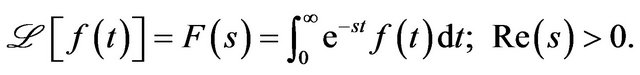
,  , in the right half complex plane, is defined by,
While we completely focus on the Laplace transform, in this paper, many of the ideas herein stem from recent work on the Sumudu transform, and studies and observations connecting the Laplace transform with the Sumudu transform through the Laplace-Sumudu Duality (LSD) for  and the Bilateral Laplace Sumudu Duality (BLSD) for
  [9-16]. Indeed, considering the
 ![]() -multiplied two-sided Laplace transform,
-multiplied two-sided Laplace transform,
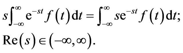
by making the parameter change s with  in the equation above we get the two-sided Sumudu transform,

Here, the constants ![]() and
and  may be finite (or) infinite, and are based on the exponential boundedness nature required on
  in the domain set

While Analyses about the properties of the Sumudu transform, transform tables, and many of its physical applications can be found in [9-12,14,16], investigations, applications, and transform tables stemming from the Natural transform can be found in [17-21]. This new integral transform combines both (one sided) Sumudu and (one sided) Laplace transforms by,
Obviously, taking,  , in the Natural transform, leads to the Laplace transform, and taking,
  , results in one sided Sumudu transform. We note that while the Natural can be bilateral like both Sumudu and Bilateral Laplace, when the variable
  is chosen positive in the definition, both
  and the variable,
 ![]() , must be positive as well, as as this ought to correct a related one sided Natural Transform defintion misprint appearing in our papers [17,18].
, must be positive as well, as as this ought to correct a related one sided Natural Transform defintion misprint appearing in our papers [17,18].
The gist and essence of this work is solving the Laplace integral equation once by differention, and by integration by parts. Divided into two major sections, this paper in Section 2 explains the various multiple shift properties connected with the Laplace transform by just differentiating the original function. The new infinite series representation of trigonometric functions related with the Laplace transform is proved in Section 3. In consequence of our formulations and derivations, three tables are provided at the end of the Section 3 ended with concluding remarks and directions for some future work. The tables are respectively covering derivatives periods for the function E  (in Table 1), 21 trignometric series expansions entries (in Table 2), and 16 main Laplace transform properties, as generated by Proposition 3 (in Table 3). Examples 1, 2, and 3 in the body of the text of Section 2, as well as Example 6 and Entry 17 of transform Table 2 in Section 3, are respectively afforded Maple graphs (see Figures 1-5), showing both the time function invoked in the corresponding example, and its resulting Laplace trasform.
2. Laplace Transforms by Function Differentiation
As stated earlier in the introduction, an ultimate goal of ours, among others, is calculating the Laplace transform of  by simple differentiation rather than usual integration. We show that we can do this, without resorting to the Adomian nor homotopy methods, ADM, and HPM, as was done in [22,23]. Along with the Laplace series definition below, some elementary properties are proved.
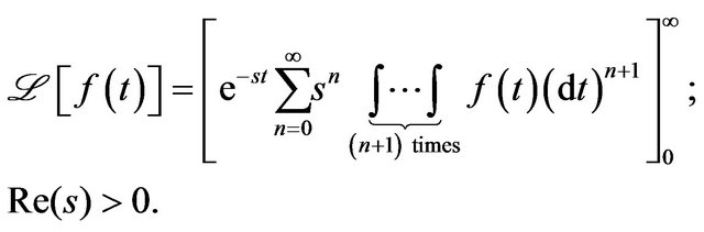
Definition The Laplace transform (henceforth designated as F(s)) of the exponential order and sectionwise continuous function , is defined by,
 (1)
(1)
Remark We observe that, from the traditional Laplace transform, taking , so that
 and
and
 , so that
 . Now using
 and
and  in Bernoulli’s integration by parts,

and noting  for n ≥ 0 Equation (1) follows.
Can’t one choose u = e−st and  for solving the Laplace integral equation by parts? The detailed answer with analysis is given in Section 3. For simplicitywe use hereafter
 .
.
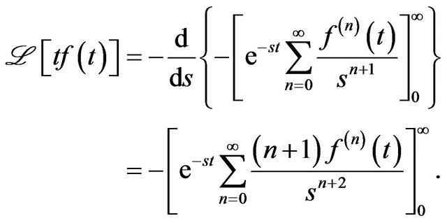
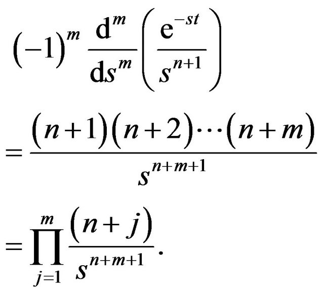
Multiple Shifts and Periodicity Results
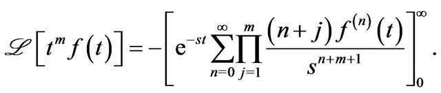
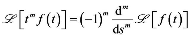
Theorem 1 The Laplace transform of  derivative of
 , with respect to
  is defined by,
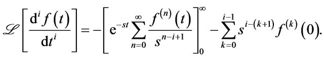
Proof. The LHS of above equation is
![]() , substituting Equation
, substituting Equation
(1) for , the proof is completed.
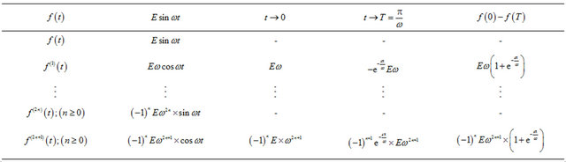
Table 1. Period function calculations.
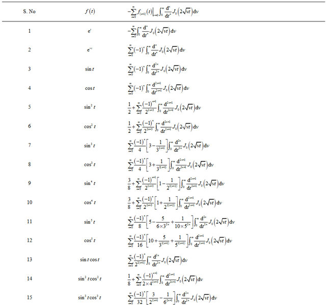
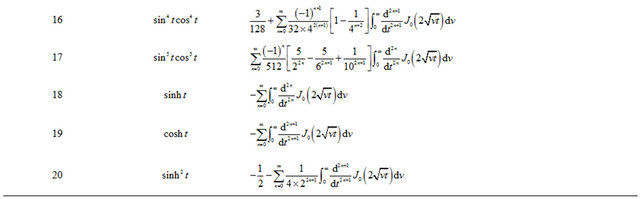
Table 2. New infinite series representation of trigonometric functions.

Table 3. Laplace transform properties with respect to the Proposition 3.
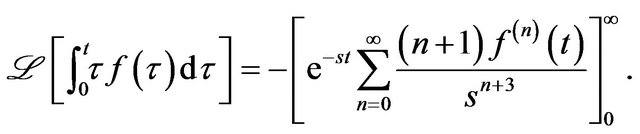
Theorem 2 The Laplace transform of  antiderivative of f(t), in the domain
  with respect to
 , is given by,
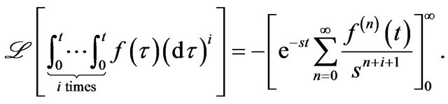
Proof. Applying Equation (1) in 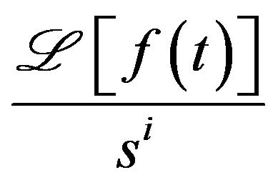 and performing the usual computations, yields the RHS of the equation above and proves out theorem.
Theorem 3 For , the Laplace transform of the function
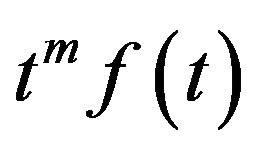 , is given by,
 (a) (b)
Figure 1. Graph of example 1. (a)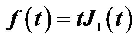 ; (b)
; (b)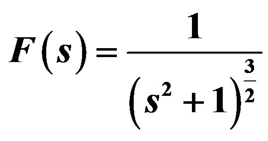 .
.
 (a) (b)
Figure 2. Graph of example 2 with a = 1, b = 2. (a) ; (b)
; (b) .
.
Proof. From the theory of Laplace transform
 , when
is given by Equation (1),
 (2)
(2)
When  in Equation (2),
 (a) (b)
Figure 3. Graph of example 3. (a)![]() ; (b)
; (b) .
.
 (a) (b)
Figure 4. Graph of example 6 with a = 5. (a) ; (b)
; (b) .
.
 (3)
(3)
When 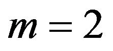 in Equation (2),
 (4)
(4)
Finally for the non-negative integer![]() , after simplifi-
, after simplifi-
 (a) (b)
 ; (b)
; (b)  .
.cation,
which yields the result of Theorem 3.
Theorem 4 The Laplace transform of the function
 , for
, for , is,
, is,

Proof. Substituting Equation (1) for  in
in
 and after the usual computations, Theorem 4 follows.
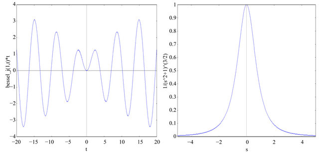
Example 1 As an application of Theorem 3, the Laplace transform of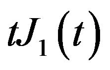 , where
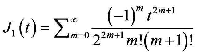 , denotes the first kind order one Bessel function, is calculated as follows, (graph shown in Figure 1),
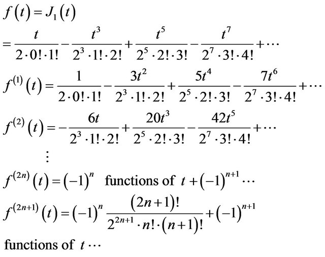
Now substituting the above derivatives in Equation (3), and after applying both the limits,  and
and
 for
for ,
,

The multiple-shift theorems that follow are useful in treating differential and integral equations with polynomial coefficients.
Example 2 The Laplace transform of 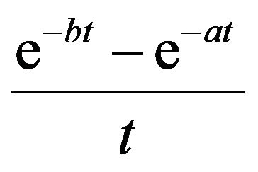 is calculated by taking,

(Figure 2), When  in Theorem 4,

So that,

Theorem 5 Let  when the
  derivative of the function
 , with respect to
  is shifted by
 , then the Laplace transform is given by,
 (5)
(5)
Proof. The proof is simple, we have
 where
where
 is given by Theorem 1.
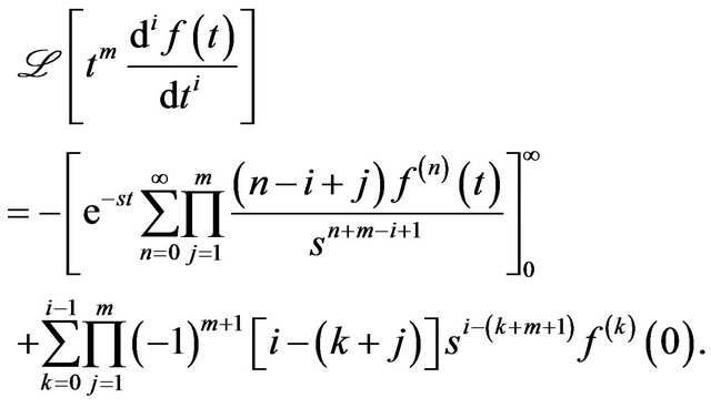
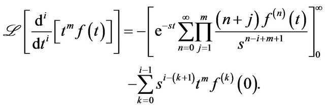
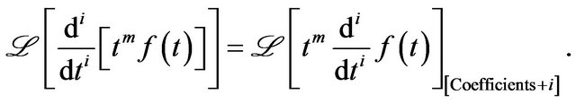
Theorem 6 For non-negative integers i and![]() , when the
, when the  derivative of the function
 , with respect to
  is shifted with
 , then the Laplace transform is given by,
 (6)
(6)
Proof. The LHS of above equation is
 and
and  are given by Theorem 1, and after proper calculations, the proof is calculated.
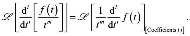
Theorem 7 For , the Laplace transform of the
  antiderivative of the function
  with respect to
  in the interval
  shifted with
 , is given by,

Proof. Applying Theorem 2 in LHS yields the RHS of the Equation above.
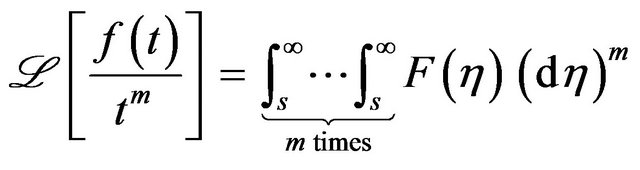
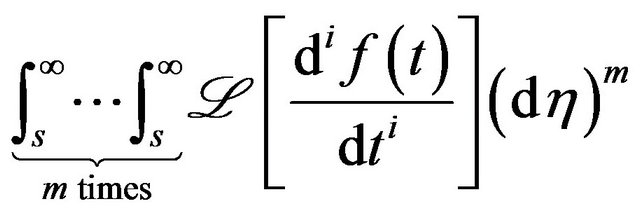
Theorem 8 The Laplace transform of the  antiderivative of the function
  with respect to
  in the interval
  shifted with
  is given by,
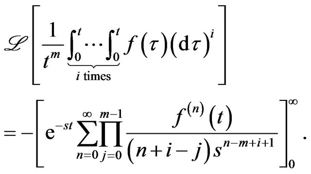
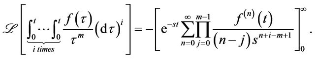
Proof. Computing the summation in the RHS of the Equation in Theorem 2 with respect to ![]() in the domain
in the domain ,
, ![]() times, yields the proof.
times, yields the proof.
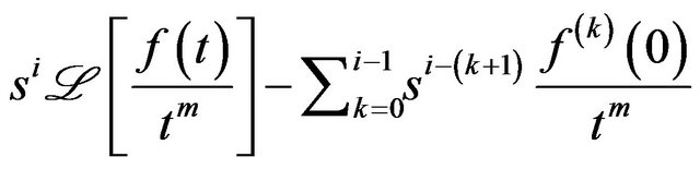
We now establish the following resultsTheorem 9 For , the Laplace transform of the
  derivative of
  with respect to
  is given by,
 (7)
(7)
Proof. Substituting Theorem 3 in
![]() .
.
Theorem 10 The Laplace transform of the 
derivative with respect to  of
of 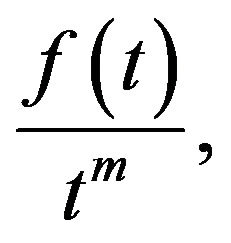 for non-negative integers,
  and
and  is given by,
 (8)
(8)
Proof. Substituting Theorem 4 in
 .
.
Example 3 Consider the function, 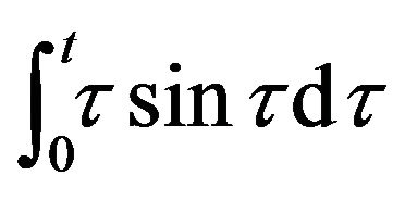 , then taking
  yields the expected derivatives,
 and,
and, ;
; . Next, for
  in Theorem 11,
Therefore (Figure 3),
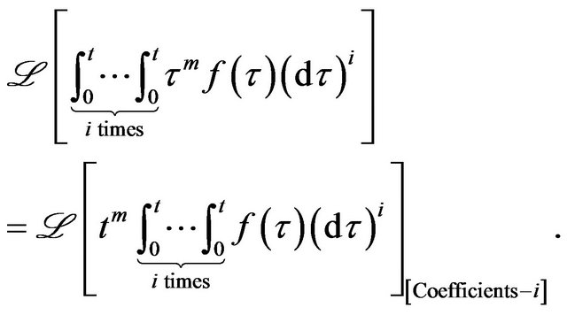
Theorem 11 For non-negative integers  and
and![]() , the Laplace transform of the
, the Laplace transform of the  antiderivative with respect to
  in the domain
  of
of , is given by,
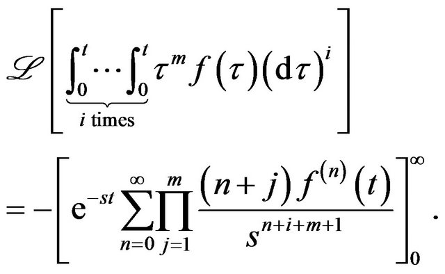
Proof. From the property of Laplace transform, the LHS of above equation is  in which Theorem 3 is substituted and simplified.
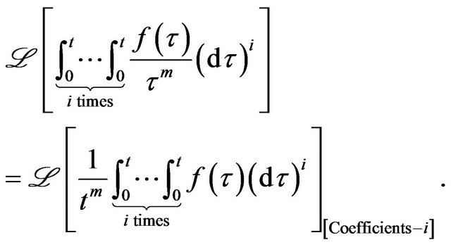
Theorem 12 The Laplace transform of the  antiderivative with respect to
  in the domain
  of
of
 , where,
  , is given by,
Proof. The proof is straightforward where we multiplied  to Theorem 4.
Example 4 Consider the function,  , which Laplace transform we can find by taking,
  yielding,
  and,
and,
 Now, since from the theorem above, for
  we have,

we consequently get,

From Theorem 5 through Theorem 12, there is no restriction on positive integers ![]() and
and , which means both can be same (or) different and either of the integer can less than (or) greater than to one another.
The Theorem 5 and the Theorem 9 varies only in the coefficients, that is the order of the derivative, the same holds for Theorem 6 and Theorem 10, again the Theorem 7 and Theorem 11 varies only in the coefficients, that is the order of the anti-derivative, similarly for Theorem 8 and 12. Hence we have the following propositions, respectively.
Proposition 1 If the function  and its
  derivative with respect to
  go to zero as
 , then,
 (9)
(9)
 (10)
(10)
Proposition 2
 (11)
(11)
 (12)
(12)
The following initial and final value, convolution, and function periodicity related theorems can be easily verified through conventional Laplace transform theory.
Theorem 13 Let the function,  be Laplace transformable, then,
 (13)
(13)
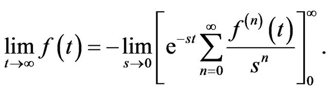 (14)
(14)
Theorem 14 The Laplace transform of the convolution of two functions , and,
  , is given by,

Theorem 15 The Laplace transform of the periodic function  with period
  so that
  , is given by,
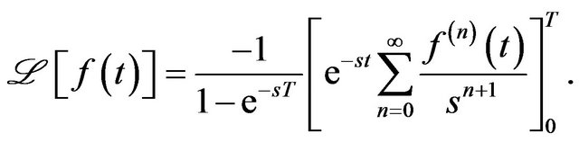
Proof. Writing Equation (1) as,
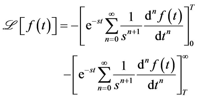
Now substituting 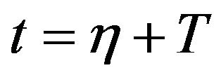 in the second infinite series of the above equation so that the limits
 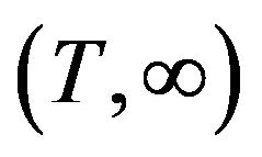 changes to
  and by having
  and after rearranging and evaluating completes the proof.
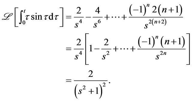
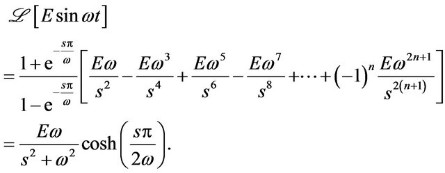
Example 5 The full sine-wave rectifier is given by the function,  with the period
 .
.
Using Theorem 15, the Laplace transform of the full sine-wave rectifier is calculated by using the entries of column 5 of Table 1,
3. Laplace Transforms by Integration by Parts
The Laplace transform of  is calculated by substituting
  in the Laplace integral transform, now by taking
  and
and  evaluating by parts gives
 . On the other hand, to calculate the Laplace transform of
![]() , we take
, we take  and
and  and after evaluation leads
 . Here we can also take u =
 and
and  again it gives the same Laplace transform. Hence, in this section, we solve the Laplace integral equation by taking,
  , and
, and , and integrating by parts. Below, the sub-scripts in say
  represents the order of integration
 ![]() in the variable
in the variable 
 .
.
Subject to some constraints we then generally haveProposition 3 The Laplace transform of a Taylor’s seriezable trigonometric function,  , is given by,
Proof. Now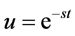 , so that
 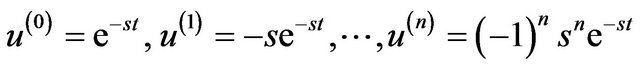 Next
Next , leads to

Substituting  and
and  in the Bernoulli’s formula of continuous integration by parts and observing
  is positive for all
  gives Proposition 3.
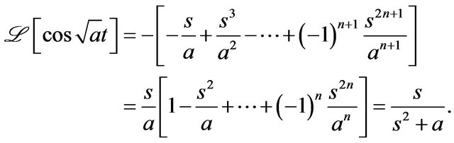
Example 6 The Laplace transform of  with non-negative integer, a, is calculated by simply integrating the function. Now, for
 ,
,
and,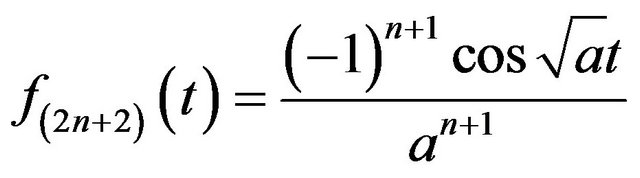 . Furthermore, in view of Proposition 3, when applying the upper and lower limits in the antiderivatives above, we get.
and , whence we get, (function and its Laplace transform in Figure 4)
We agree that constants and polynomials cannot be Laplace transformed with the Proposition 3, since the continuous integration of constant and polynomials with respect to  does not converge anywhere when
  and
and .
.
3.1. New Infinite Series Representation for Trig Functions
In the Proposition 3 the limitations of  to be Taylor’s seriezable trigonometric function is acceptable only on a theoritical point of view, from the evaluation of Laplace transform of trigonometric functions vice-versa of Definition of Section 2 and Proposition 3. On the other hand, we show under what condition the Proposition 3 exists? Definitely the answer would be by finding the inverse Laplace transform of Proposition 3.
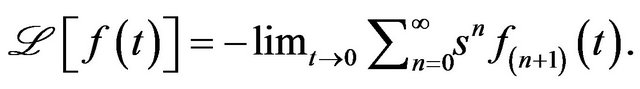
For simplicity’s sake, re-writing the Proposition 3, is akin to evaluating the limits and representing,  , in Proposition 3. The Laplace transform of Taylor’s seriezable trigonometric function
  is simply defined by,

The inverse Laplace transform of Proposition 3 would be same as inverse Laplace transform of the above equation, and hence it is enough to find the inverse Laplace transform of .
.
For a start up, when  in
in  the inverse Laplace transform of
  would be
  which is Dirac delta function [2] since,
 .
.
Again when  in
in  the inverse Laplace transform of s is given by the first derivative of Dirac delta function with respect to
 ,
, . In particular, readers are invited to consider connected relation to Dirac delta function but in the Sumudu transform context (see Equations (2.19), (2.20), (4.18), and (4.20) in [9]). In general, the inverse Laplace transform of
  is given by
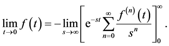
 , since
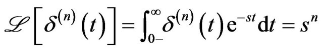 . In all cases upto the n-th derivative the initial value theorem is undefined for
  and
and  leads of course to the study of generalized functions (see [2], and references therein for more details).
We prove the inverse Laplace transform of singular functions that satisfy the Tauberian (initial value) theorem in the following proposition where the trigonometric functions are represented in new infinite series, where coefficients are calculated by integrating the function, [24].
Proposition 4 The necessary condition for the existence of Proposition 3 (and hence the above equation) is that, the Taylor seriezable trigonometric function  can be expressed as,
Proof. Taking inverse Laplace transform of
 (15)
(15)
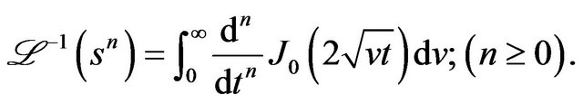
In [14] the Bilateral Laplace Sumudu Duality (BLSD) was established. the inverse Laplace transform of  is given by (see Equation (5.10) in [14]),
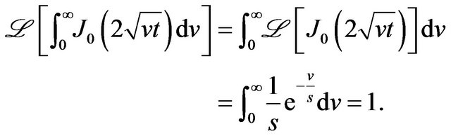 (16)
(16)
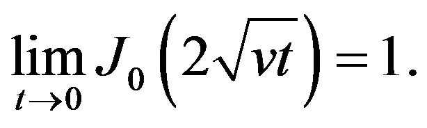
Thus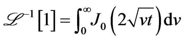 , here the
 is the first kind Bessel’s function of order zero. And this particular function will play the major role in the exponential kerneled integral transforms (see Equations (30) through (35) in [20]). And the Laplace transform is taken with respect to
 , since v and
  are independent, the permissibility of interchange of order of integration is considered in favour. Though the function
 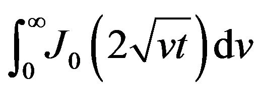 gives no meaning (as becomes zero when evaluated) but as per the Laplace (integral) transform point of view this is worth (see Theorem 5.1. Equation (5.8) in [14]). By having,
 (17)
(17)
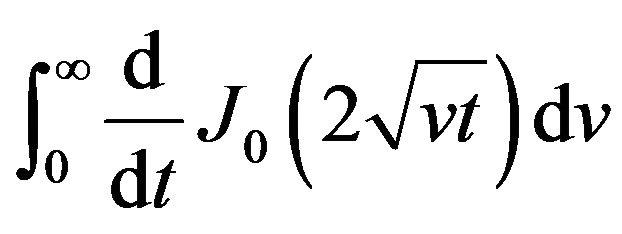
The Laplace transform of the first derivative of
 with respect to
  is
is  and with the help of Equations (16) and (17),
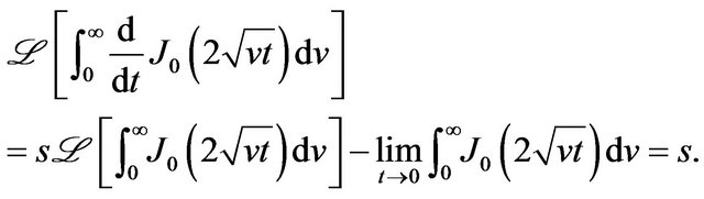 (18)
(18)
Therefore the inverse Laplace transform of ![]() is
is
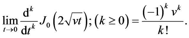
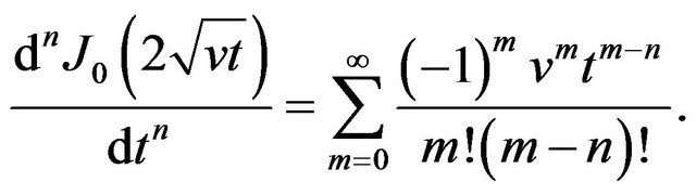
 . In general, from the Laplace transform of the
 ![]() derivative of function with respect to
derivative of function with respect to ,
,
 (19)
(19)
But,
 (20)
(20)
Finally from Equations (19) and (20),
 (21)
(21)
Since the second part of right hand side of Equation (21) is zero,
 (22)
(22)
Substituting Equation (22) in Equation (15) for  completes the proof of Proposition 4.
Thus, the function  from the Equation (20) satisfies the initial value theorem (unlike Dirac delta function) which is zero. To concretize ideas, we give the following example.
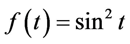
Example 7 Consider the function , then
 ,
, 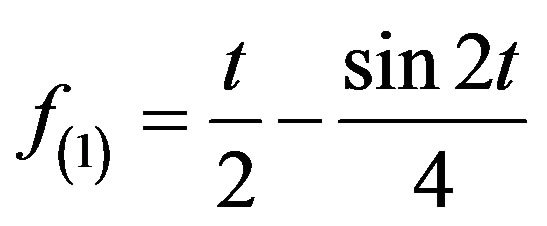 ,
, 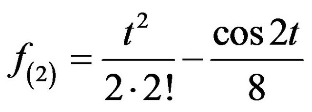 ,
,
 ,
, 
 , and,
 . Applying Proposition 4, as t tends to zero, all the
  and
and
 and since
 ![]() is the common factor,
is the common factor,
 , the function,
  , can be written in the new infinite series as,

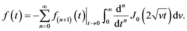
From Equation (22), it is wothy to note that the Laplace transform of the integral of ![]() derivative of
derivative of  with respect to t, in the domain
  with respect to v, is simply the s power the order of the derivative of
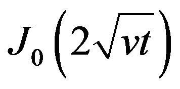 .
.
Along with that of the function,  , in light of this new infinite series Proposition 4, Table 2 gives all new infinite series expansions of basic trigonometric functions. The extra factor in the infinite series of entries 5, 6, 9, 10, 14, 16, 20 and 21 are common for all
  while integrating. Furthermore, the following expression is easily derivable from the Bessel’s function,
Therefore, the Laplace transform of  can be calculated through,
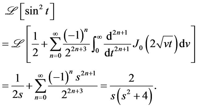
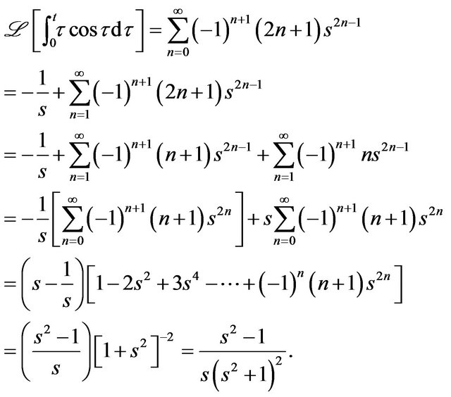
Entry 17 of Table 2 has the following Laplace transform (shown in Figure 5),
3.2. LaplaceTransform Properties in View of Proposition 3
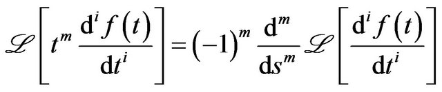
The Laplace transform of multiple shifts functions can readily be derived with the help of Proposition 3. Since the derivation of the various properties are straightforward and similar to the theorems of Section 2.1, we give directly the Laplace transform of shifted functions, based on Proposition 3 in Table 3 where ![]() and i are non-negative integers.
and i are non-negative integers.
Example 8 The Laplace transform of the function, 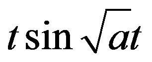 , is obtained by simply integrating
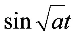 thus
thus ,
,  ,
,  ,
,
 ,
, .
.
When,  , in entry 3 of Table 3,

Therefore, when , and
, and ,
, 
and  yielding,
Example 9 The Laplace transform of  is calculated by integrating cost. Now,
  ,
,  ,
,
 and,
and,
 . Now, for,
  , and,
 and,
and, .
.
Finally, with  in the entry 4 of Table 3,
So that,

Example 10 The Laplace transform of, 
is calculated. For,  , after taking limits, we get,
  Hence, applying the formula with,
  , in entry 11 of Table 3,

We consequently then have,
It is important to note that with respect to the entries 5 and 9 (and entries 6 and 10) of Table 3, the proposition 1 Equation (9) (and Equation (10)) holds true. Similarlly with respect to the entries 7 and 11 (and entries 8 and 12) of Table 3, the proposition 2 Equation (11) (and Equation (12)) remains the same.
3.3. Concluding Remarks and Future Work
As far as the Section 2 is concerned, when the function is Laplace transformed by differentiation, then the inverse Laplace is automatically an integration process. Having worked with various examples, our proposed methods lead to exact solutions. A remaining open query is that of defining the inverse for the Laplace transform by using similar tools and processes as in Proposition 3. But in view of the concept of Section 2 above, Laplace and inverse Laplace transform are the respective reciprocal processes of differentiation and integration of the function.
If so, then with the Proposition 3, the inverse Laplace transform will be the process of differentiating. For example consider the function , its Laplace transform by the Proposition 3 is given by
which gives . Hence for finding the original function, when equating the coefficients of identical powers of
 ![]() with Proposition 3, we get
with Proposition 3, we get  As the sub-scripts denote the order of integration. Now by differentiating
  times, one should get the infinite series of the function, cost as entry 4 of Table 2.
As part of some future works in this regard, we aspire to pursing working schemes of this paper, and establishing more comprehensive tables as was done for the Sumudu transform in [10], and for the Natural transform in [17]. With this said, it is perhaps research worthy, in the near future, to put all considered aspects in the framework and applications of the theory of reproducing kernels [25].
4. Acknowledgements
The Authors wish to acknowledge and thank the AM Editorial Board, as well as SCRIP Grants Committee, for helping defray a major part (75%) of the processing charges of this article. We also thank the referees and AM staff for constructive comments that helped improve the structural flow of the paper.
REFERENCES
- L. Debnath and D. Bhatta, “Integral Transforms and Their Applications,” 2nd Edition, C. R. C. Press, London, 2007.
- P. P. G. Dyke, “An Introduction to Laplace Transform and Fourier Series,” Springer-Verlag, London, 2004.
- A. Erdélyi, W. Magnus, F. Oberhettinger and F. G. Tricomi, “Tables of Integral transform,” Vol. 1, McGrawHill, New York, Toronto, London, 1954.
- M. Rahman, “Integral Equations and Their Applications,” WIT Press, Boston, 2007.
- J. L. Schiff, “Laplace Transform Theory and Applications,” Springer, Auckland, 2005.
- M. R. Spiegel, “Theory and Problems of Laplace Transforms,” Schaums Outline Series, McGraw-Hill, New York, 1965.
- W. T. Thomson, “Laplace Transformation Theory and Engineering Applications,” Prentice-Hall Engg Design Series, Printice-Hall Inc., New York, 1950.
- D. V. Widder, “The Laplace Transform,” Oxford University Press, London, 1946.
- F. B. M. Belgacem, A. A. Karaballi and S. L. Kalla, “Analytical Investigations of the Sumudu Transform and Applications to Integral Production Equations,” Mathematical Problems in Engineering (MPE), Vol. 2003, No. 3, 2003, pp. 103-118.
- F. B. M. Belgacem and A. A. Karaballi, “Sumudu Transform Fundamental Properties Investigations and Applications,” Journal of Applied Mathematics and Stochastic Analysis (JAMSA), 2005, Article ID: 91083.
- F. B. M. Belgacem, “Introducing and Analysing Deeper Sumudu Properties,” Nonlinear Studies Journal (NSJ), Vol. 13, No. 1, 2006, pp. 23-41.
- F. B. M. Belgacem, “Applications of Sumudu Transform to Indefinite Periodic Parabolic Equations,” In: Proceedings of the 6th International Conference on Mathematical Problems & Aerospace Sciences (ICNPAA 06), Chap. 6, Cambridge Scientific Publishers, Cambridge, 2007, pp 51-60.
- F. B. M. Belgacem, “Sumudu Applications to Maxwell’s Equations,” PIERS Online, Vol. 5, No. 4, 2009, pp 355- 360. doi:10.2529/PIERS090120050621
- F. B. M. Belgacem, “Sumudu Transform Applications to Bessel’s Functions and Equations,” Applied Mathematical Sciences, Vol. 4, No. 74, 2010, pp. 3665-3686.
- M. G. M. Hussain and F. B. M. Belgacem, “Transient Solutions of Maxwell’s Equations Based on Sumudu Transform,” Journal of Progress in Electromagnetics Research (PIER), Vol. 74, 2007, pp. 273-289. doi:10.2528/PIER07050904
- M. A. Rana, A. M. Siddiqui, Q. K. Ghori and R. Qamar, “Application of He’s Homotopy Perturbation Method to Sumudu Transform,” International Journal of Nonlinear Sciences and Numerical Simulation, Vol. 8, No. 2, 2007, pp. 185-190.
- F. B. M. Belgacem and R. Silambarasan, “Theory of the Natural Transform,” Mathematics in Engineering, Science and Aerospace (MESA) Journal, Vol. 3, No. 1, 2012, pp. 99-124.
- F. B. M. Belgacem and R. Silambarasan, “Maxwell’s Equations Solutions by Means of the Natural Transform,” Mathematics in Engineering, Science and Aerospace (MESA) Journal, Vol. 3, No. 3, 2012, pp. 313-323.
- F. B. M. Belgacem and R. Silambarasan, “The Generalized n-th Order Maxwell’s Equations,” PIERS Proceedings, Moscow, 19-23 August 2012, pp. 500-503.
- F. B. M. Belgacem and R. Silambarasan, “Advances in the Natural Transform,” AIP Conference Proceedings, Vol. 1493, 2012, pp. 106-110. doi:10.1063/1.4765477
- R. Silambarasan and F. B. M. Belgacem, “Applications of the Natural Transform to Maxwell’s Equations,” PIERS Proceedings, Suzhou, 12-16 September 2011, pp. 899- 902.
- S. Abbasbandy, “Application of He’s Homotopy Perturbation Method for Laplace Transform,” Journal of Chaos, Solitons and Fractals, Vol. 30, No. 5, 2006, pp. 1206- 1212. doi:10.1016/j.chaos.2005.08.178
- E. Babolian, J. Biazar and A. R. Vahidi, “A New Computational Method for Laplace Transform by Decomposition Method,” Journal of Applied Mathematics and Computation, Vol. 150, No. 3, 2004, pp. 841-846. doi:10.1016/S0096-3003(03)00312-6
- C. J. Efthimiou, “Trigonometric Series via Laplace Transform,” 2007. http://arxiv.org/abs/0707.3590v1
- S. Saitoh, “Theory of Reproducing Kernels: Applications to Approximate Solutions of Bounded Linear Operator Equations on Hilbert Spaces,” American Mathematical Society Translations, Vol. 230, No. 2, 2010, pp. 107-134.
NOTES
*Corresponding author.