Applied Mathematics
Vol.4 No.1(2013), Article ID:27195,6 pages DOI:10.4236/am.2013.41011
Synchronization of Chaotic Energy Resource System
School of Physics and Optoelectronic Engineering, Nanjing University of Information Science & Technology, Nanjing, China
Email: tbwang@nuist.edu.cn
Received October 15, 2012; revised November 15, 2012; accepted November 23, 2012
Keywords: Unilateral Coupling Method; Coupling Coefficient; Chaos Synchronization; Synchronizing Time
ABSTRACT
Taking a four-dimensional energy resources demand-supply system between the East and West of China, this paper discusses its chaotic behavior, and via the unilateral coupling method we lead the system to synchronization successfully. But not all the values of coupling coefficient can lead to synchronization. The values of coupling coefficient have a range. By calculating the maximal relative Lyapunov exponents’ spectrum, we gained the value range of coupling coefficients. Within the value range, the two coupling systems can achieve synchronization, otherwise can’t. Further more, the values of coupling coefficient are in connection with the chaos synchronizing time. At last, we get the relationship of coupling coefficients and chaos synchronizing time.
1. Introduction
Generally, designing a controller to force a system to imitate the behavior of another chaotic system is called synchronization [1]. Chaos synchronization and chaos control have been applied broadly in many fields such as in biological systems, chemical reactions, information processing, especially in secure communication area [2]. There are plenty of methods have been proposed to achieve chaos synchronization, for example, sliding mode control [3], linear control [4], adaptive control [5], digital redesign control [6] and so on.
Nowadays, many countries attach importance to the exploitation and utilization of clear energies, and develop low carbon economy. Considering renewable energy resources, based on a three dimensional system, gained a four-dimensional energy resources demand-supply system between east and west in China by adding a new variable [7]. This paper discusses the chaotic behavior of it, and uses the unilateral coupling method achieving chaos synchronization successfully. By means of calculating the maximal relative Lyapunov exponents, we get the value range of the coupling coefficient. Also, we get the relationship of coupling coefficient and chaos synchronizing time.
2. The Unilateral Coupling Method
In 1993, K. Pyragas proposed a way to control a nonlinear system, which is called the error variable negative feedback control also the unilateral coupling method [8].
Supposing there are two chaotic systems:  ,
,  , which are defined by following dynamic functions:
 , (1)
, (1)
where K(X−Y) is a coupling item,  is coupling coefficient, which are equal upon each variable and take positive values commonly, i.e.
  . When the parameters of the two systems are matched, as long as take an appropriate coupling coefficient K, the two systems can achieve synchronization. This method won’t change the system’s initial dynamic characteristic, because the coupling item K(X – Y) = 0 after synchronization. The characteristic of the method is we needn’t analyze the system in advance. Further more, we can confirm the domain of the coupling coefficient by calculating.
3. Discussion of the Energy Resource Demand-Supply System between East and West in China
Adding a new variable to a three dimensional energy resource system, gained a four dimensional energy resources demand-supply system between east and west in China, which is defined by the functions below [7]:
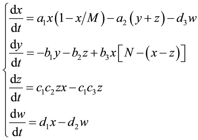 (2)
(2)
where x(t) is the energy resource shortage in A region, y(t) expresses the energy resources supply increment in B region, z(t) the energy resources import in A region, w(t) is the amount of renewable energy resources in A region; ai, bi, ci, di and M, N are positive real constants [7]. When M = 1.8, N = 1, a1 = 0.1, a2 = 0.15, b1 = 0.06, b2 = 0.082, b3 = 0.07, c1 = 0.2, c2 = 0.5, d1 = 0.1, d2 = 0.06, d3 = 0.07, and the initial condition  , the system can generate complex chaotic attractor, the numerical simulation is shown in Figure 1, from which we can see the system has an abundant chaotic behavior.
4. Chaos Synchronization
4.1. Realization of Chaos Synchronization
According to the unilateral coupling method, we define the energy resource system (3), which is described as follows:
 (3)
(3)
whose initial condition x1(0), x2(0), x3(0), x4(0) takes a random real constant from (0, 1) respectively.
Copying a system and adding coupling items, we obtain the system (4) defined below:
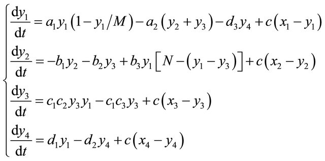
(4)
where c is the coupling coefficient, and the initial condi-
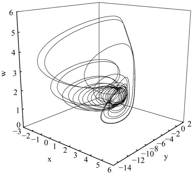
Figure 1. When M = 1.8, N = 1, a1 = 0.1, a2 = 0.15, b1 = 0.06, b2 = 0.082, b3 = 0.07, c1 = 0.2, c2 = 0.5, d1 = 0.1, d2 = 0.06, d3 = 0.07, and the initial condition [x(0) y(0) z(0) w(0)] = [0.82 0.29 0.48 0.1], the chaotic attractor of energy resource system (2).
tion y1(0), y2(0), y3(0), y4(0) also takes a random real constant from (0, 1) respectively.
The errors of corresponding variables between system (3) and system (4) are denoted as
 , (5)
, (5)
and
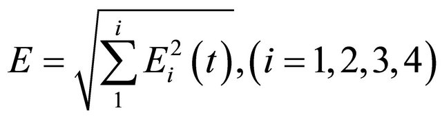 (6)
(6)
which express the situation of chaos synchronization. When Ei(t) and E equals to zero and then stable over time, we can say systems (3) and (4) have achieved synchronization, otherwise not. Randomly, chose c = 2, the errors Ei(t) is shown as Figure 2, and the errors E is shown in Figure 3.
Figure 2 (or Figure 3) indicates clearly that when c = 2, Ei(t) (or E) tends to zero immediately and then stable, in other words, systems (3) and (4) achieved synchronization quickly. Thus, via the unilateral coupling method, we have made two systems achieve synchronization successfully.
But not all the values of coupling coefficient can lead to synchronization according to the following discussion.
4.2. Confirmation of Coupling Coefficients
Then let c = 0.01, the numerical simulation of the errors Ei(t) is shown as Figure 4, the errors E is shown as Figure 5. The Bifurcation diagram under various coupling coefficient from 0 - 0.1 is shown as Figure 6.
From Figure 4 (or Figure 5), we can clearly see that when c = 0.01, Ei(t) (or E) vibrates desultorily all the time, namely this value of coupling coefficient c won’t
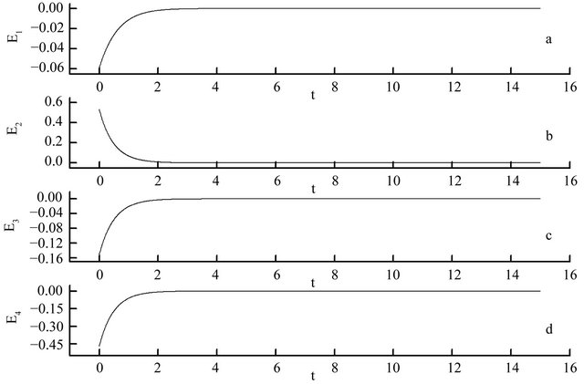
Figure 2. When the coupling coefficient c = 2, the errors of corresponding variables between systems (3) and (4), Ei(t), varies over time.

Figure 3. When the coupling coefficient c = 2, the errors of corresponding variables between systems (3) and (4), E, varies over time.
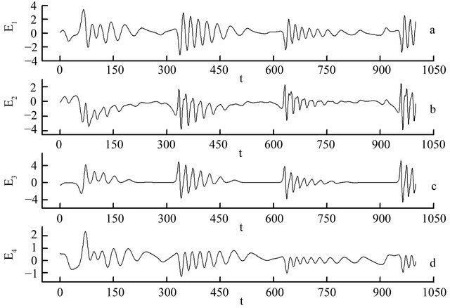
Figure 4. When the coupling coefficient c = 0.01, the errors of corresponding variables between systems (3) and (4), Ei(t), varies over time.
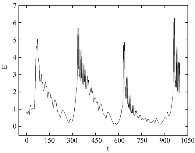
Figure 5. When the coupling coefficient c = 0.01, the errors of corresponding variables between system (3) and system (4), E, varies over time.
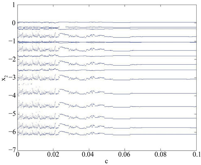
Figure 6. The relation between coupling coefficients and x2 of the system (3).
lead the two systems to synchronization.
So, we conclude not all the values of coupling coefficient can lead the two systems to synchronization; Values of c have a domain, values in which can make the two systems achieve synchronization, values outside it are not appropriate. By calculating the maximal relative Lyapunov exponents’ spectrum, we can get the value range of c.
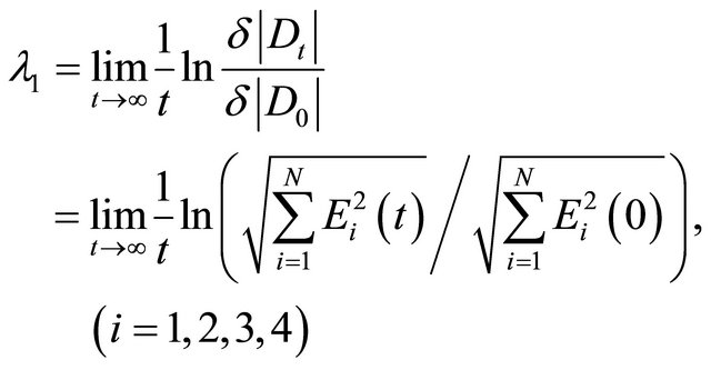
In a chaotic system, the maximal Lyapunov exponent is a quantity characterizes the rate of separation of infinitesimally close trajectories, also the quantity indicates the strength of butterfly effect. In coupled systems, when maximal relative Lyapunov exponent is less than zero, the two systems will achieve synchronization, otherwise won’t [9]. The definition of maximal relative Lyapunov exponent [9] is
 (7)
(7)
where Dt is the distance of the two system’s trajectories at the time of t, D0 is the distance of the two system’s trajectories at the initial time, Ei(t) the error of corresponding variables between systems at t moment, Ei(0) the error of corresponding variables between systems initially, N is dimension. The numerical relation between coupling coefficients and the maximal relative Lyapunov exponents is shown in Figure 7.
As shown in Figure 6, when c > 0.043, the maximal relative Lyapunov exponent is less than zero, thus systems (3) and (4) can achieve synchronization successfully, while c < 0.043, the maximal relative Lyapunov exponent is more than zero, the two systems can’t achieve synchronization. So when c = 0.01, the maximal relative Lyapunov exponent is more than zero, the two systems haven’t achieved synchronization, as shown in Figure 4 (or Figure 5).
4.3. The Relation between Coupling Coefficients and Synchronizing Time
When c = 0.2, the errors Ei(t) is shown as Figure 8, the errors E is shown as Figure 9.
Comparing Figure 7 (or Figure 8) and Figure 4 (or Figure 5), we see that when c = 2, the time achieving synchronization is shorter than the instance of c = 0.2.
In fact, sometime we need achieve synchronization immediately, while sometime we need transit a certain time and then achieve synchronization. So, the choice of a coupling coefficient’s value is crucial, and it’s neces-
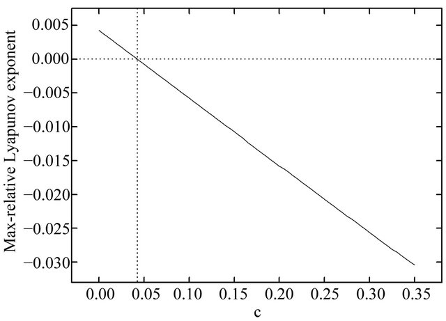
Figure 7. The relation between coupling coefficients and the maximal relative Lyapunov exponents of systems (3) and (4).
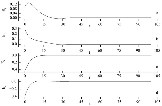
Figure 8. When the coupling coefficient c = 0.2, the errors of corresponding variables between systems (3) and (4), Ei(t), varies over time.

Figure 9. When the coupling coefficient c = 0.2, the errors of corresponding variables between systems (3) and (4), E, varies over time.
sary to discuss the relation between coupling coefficients and the time achieving synchronization.
Figure 10 presents the relation between coupling coefficients and the synchronizing time. Though there comes some gurgitation, but generally, the bigger coupling coefficient is, the shorter two systems achieve synchronization. It is an important conclusion, in practice, we can choose an appropriate coupling coefficient according to demand.
5. Conclusion
Based on a four-dimensional energy resource demandsupply system between the East and West of China, via numerical simulation, this paper discusses its chaotic behavior, and uses the unilateral coupling method achiev-
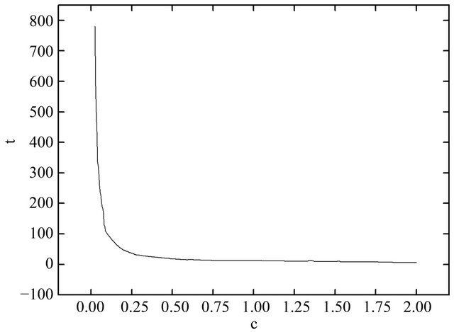
Figure 10. The relation between coupling coefficients and synchronizing time of systems (3) and (4).
ing the chaos synchronization. By computing the maximal relative Lyapunov exponents’ spectrum of systems (3) and (4), we gained the value range of coupling coefficients. When coupling coefficient c > 0.043, the maximal relative Lyapunov exponent is less than zero, thus the two systems can achieve synchronization sucessfully, while c < 0.043, the maximal relative Lyapunov exponent is more than zero, the two systems can’t achieve synchronization. At last, we get the relationship between coupling coefficients and synchronizing time, i.e. the greater coupling coefficient is, the shorter systems achieve synchronization.
REFERENCES
- C. F. Huang, K. H. Cheng and J. J. Yan, “Robust Chaos Synchronization of Four-Dimensional Energy Resource Systems Subject to Unmatched Uncertainties,” Communications in Nonlinear Science and Numerical Simulation, Vol. 14, No. 6, 2009, pp. 2784-2792. doi:10.1016/j.cnsns.2008.09.017
- J. A. Lu, X. Q. Wu and J. H. Lu, “Synchronization of a Unified Chaotic System and the Application in Secure Communication,” Physics Letters, Vol. 305, No. 6, 2002, pp. 365-370. doi:10.1016/S0375-9601(02)01497-4
- S. A. Ammour, S. Djennoune and M. Bettayed, “A Sliding Mode Control for Linear Fractional Systems with Input and State Delays,” Communications in Nonlinear Science and Numerical Simulation, Vol. 14, No. 5, 2009, pp. 2310-2318. doi:10.1016/j.cnsns.2008.05.011
- B. L. Feng, B. Han and H. H. Dong, “Integrable Couplings and Hamiltonian Structures of the L-Hierarchy and the T-Hierarchy,” Communications in Nonlinear Science and Numerical Simulation, Vol. 13, No. 7, 2008, pp. 1264- 1271. doi:10.1016/j.cnsns.2007.02.004
- S. Bowong, “Adaptive Synchronization between Two Different Chaotic Dynamical Systems,” Communications in Nonlinear Science and Numerical Simulation, Vol. 12, No. 6, 2007, pp. 976-985. doi:10.1016/j.cnsns.2005.10.003
- S. M. Guo, L. S. Shieh, G. Chen and C. F. Lin, “Effective Chaotic Orbit Tracker: A Prediction-Based Digital Redesign Approach,” IEEE Transactions on Circuits and Systems, Vol. 47, No. 11, 2000, pp. 1557-1560. doi:10.1109/81.895324
- M. Sun, Q. Jia and L. X. Tian, “A New Four-Dimensional Energy Resources System and Its Linear Feedback Control,” Chaos Solitons & Fractals, Vol. 39, No. 1, 2009, pp. 101-108. doi:10.1016/j.chaos.2007.01.125
- G. R. Chen, et al., “From Chaos to Order,” World Scientific Publishing, Singapore City, 1997.
- T. B. Wang, T. F. Qin and G. Z. Chen, “Coupled Synchronization of Hyperchaotic Systems,” Acta Physica Sinica, Vol, 50, No. 11, 2001, pp. 1851-1855.