Applied Mathematics
Vol.3 No.8(2012), Article ID:21491,8 pages DOI:10.4236/am.2012.38132
An Asymptotic-Fitted Method for Solving Singularly Perturbed Delay Differential Equations
1Bahir Dar University, Bahir Dar, Ethiopia
2National Institute of Technology, Warangal, India
Email: *awoke248@yahoo.com, ynreddy@nitw.ac.in
Received June 9, 2012; revised July 11, 2012; accepted July 18, 2012
Keywords: Asymptotic-Fitted Scheme; Delay-Differential Equations; Singular Perturbation; Boundary Layer
ABSTRACT
In this paper, we presented an asymptotic fitted approach to solve singularly perturbed delay differential equations of second order with left and right boundary. In this approach, the singularly perturbed delay differential equations is modified by approximating the term containing negative shift using Taylor series expansion. After approximating the coefficient of the second derivative of the new equation, we introduced a fitting parameter and determined its value using the theory of singular Perturbation; O’Malley [1]. The three term recurrence relation obtained is solved using Thomas algorithm. The applicability of the method is tested by considering five linear problems (two problems on left layer and one problem on right layer) and two nonlinear problems.
1. Introduction
The problems in which the highest order derivative term is multiplied by a small parameter are known to be perturbed problems and the parameter is known as the perturbation parameter. A singularly perturbed differentialdifference equation is an ordinary differential equation in which the highest derivative is multiplied by a small parameter and involving at least one delay or advance term. Recently by constructing a special type of mesh, so that the term containing delay lies on nodal points after discretization R. N. Rao, P. P. Chakravarthy [2], presented a fourth order finite difference method for solving singularly perturbed differential difference equations. H. S. Prasad and Y. N. Reddy [3] considered Differential Quadrature Method for finding the numerical solution of boundary-value problems for a singularly perturbed differential-difference equation of mixed type. In recent papers [4-8] the terms negative or left shift and positive or right shift have been used for delay and advance respectively.
The differential-difference equation plays an important role in the mathematical modeling of various practical phenomena in the biosciences and control theory. Any system involving a feedback control will almost always involve time delays. These arise because a finite time is required to sense information and then react to it. For a detailed discussion on differential-difference equation one may refer to the books and high level monographs: Bellen [9], Driver [10], Bellman and Cooke [11].
In [12], similar boundary value problems with solutions that exhibit rapid oscillations are studied. Based on finite difference scheme, fitted mess and B-spline technique, piecewise uniform mess an extensive numerical work had been initiated by M. K. Kadalbajoo and K. K. Sharma in their papers [4-8] for solving singularly perturbed delay differential equations.
It is well known that the classical methods fail to provide reliable numerical results for such problems (in the sense that the parameter and the mess size cannot vary independently). Lange and Miura [13-15] gave asymptotic approaches in the study of class of boundary value problems for linear second order differential difference equations in which the highest order derivative is multiplied by small parameter. The effect of small shifts on the oscillatory solution of the problem has been discussed in [14].
The aim of this paper is to provide an asymptotic-fitted method to solve singularly perturbed delay differential equations of second order with left and right boundary. In this technique, by approximating the term containing negative shift by Taylor series, we modify the singularly perturbed delay differential equations. We introduce a fitting parameter on the highest order derivative term of the new equation. The fitting parameter is to be determined from the upwind scheme using the theory of singular Perturbation; O’Malley [1]. Finally, we obtain a three term recurrence relation that can be solved using Thomas algorithm. The applicability of the method is tested by considering five problems which have been widely discussed in literature (two linear problems on left layer, one linear problem on right layer and two nonlinear problems).
2. The Asymptotic-Fitted Scheme
To describe the method, we first consider a linear singularly perturbed delay differential two-point boundary value problem of the form:
 (1)
(1)
with
 (2a)
(2a)
and
 ; (2b)
where e is a small positive parameter ,
,  are bounded functions in
  and
and  are known constants. Furthermore, we assume that
  throughout the interval [0,1], where M is a positive constant. Under these assumptions, (1) has a unique solution y(x) which in general, displays a boundary layer of width O(e) at
 .
.
Approximating  by the Taylor expansion, we have
 (3)
(3)
Substituting Equation (3) in to Equation (1), we get
 (4a)
(4a)
 (4b)
(4b)
For appropriate choices of ![]() such that
such that
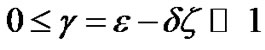 , where
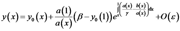
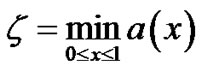 , from the theory of singular perturbations it is known that the solution of (4) and (2) is of the form [O’ Malley [1]; pp. 22-26].
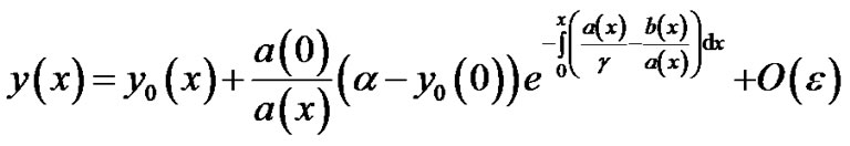 (5)
(5)
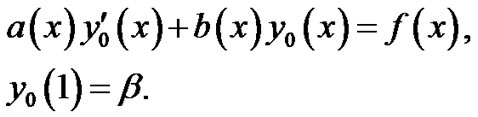
where  is the solution of
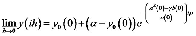
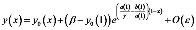
By taking the Taylor’s series expansion for a(x) and b(x) about the point “0” and restricting to their first terms, (5) becomes,
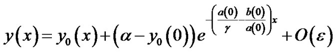 (6)
(6)
Now we divide the interval [0, 1] into N equal parts with constant mesh length h. Let 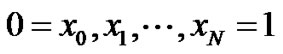 be the mesh points. Then we have
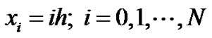 .
.
From (6) we have
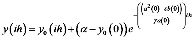 (7)
(7)
and
 (8)
(8)
where .
.
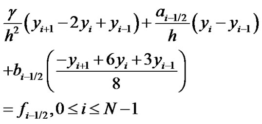
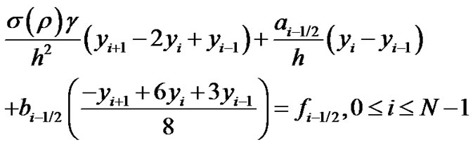
The special second order scheme corresponding to Equation (4b) [one can see [2]] is:
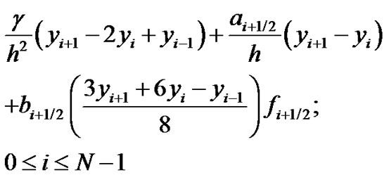 (9)
(9)
Now, we introduce a fitting factor  in the above scheme (9)
 (10)
(10)
with y(0) = a and y(1) = b.
The fitting factor s(r) is to be determined in such a way that the solution of (10) converges uniformly to the solution of (1)-(2).
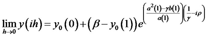
Multiplying (10) by h and taking the limit as h ® 0; we get
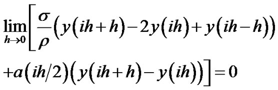 (11)
(11)
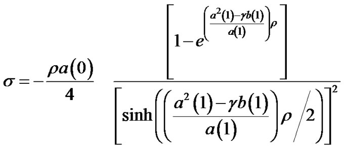
By substituting (7) in (11) and simplifying, we get the constant fitting factor
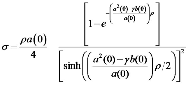 (12)
(12)
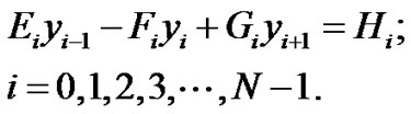
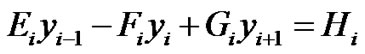
The equivalent three term recurrence relation of Equation (10) is given by:
 ;
; (13)
(13)
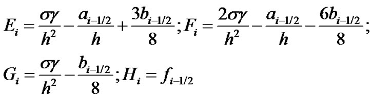
where,
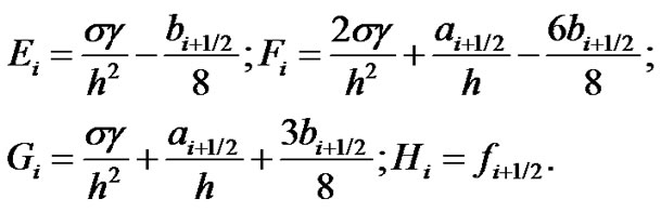
This gives us the tri diagonal system which can be solved easily by Thomas Algorithm.
Thomas Algorithm
A brief discussion on solving the three term recurrence relation using Thomas algorithm which also called Discrete Invariant Imbedding (Angel & Bellman [17]) is presented as follows:
Consider the scheme given in (13):
subject to the boundary conditions
 ; and
; and  (13a)
(13a)
We set
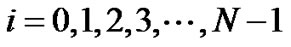
 for
for  (13b)
(13b)
where  and
and 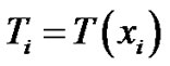 which are to be determined.
From (13b), we have
 (13c)
(13c)
By substituting (13c) in (13), we get
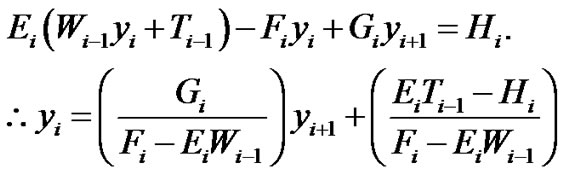 (13d)
(13d)
By comparing (13d) and (13b), we get the recurrence relations
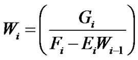 (13e)
(13e)
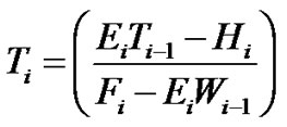 . (13f)
To solve these recurrence relations for
 , we need the initial conditions for
  and
and . For this we take
 . We choose
  so that the value of
 . With these initial values, we compute
  and
and ![]() for
for  from (13e)-(13f) in forward process, and then obtain
  in the backward process from (13b) and (13a).
The conditions for the discrete invariant embedding algorithm to be stable are (see [16] & [17]):
 ,
,  ,
,  and
and  (13g)
(13g)
In this method, if the assumptions  and
and  hold, one can easily show that the conditions given in (13g) hold and thus the invariant imbedding algorithm is stable.
3. Right-End Boundary Layer
We now assume that  throughout the interval [0, 1], where M is some negative constant. This assumption merely implies that the boundary layer for Equation (1)-(2) will be in the neighborhood of x = 1. From the theory of singular perturbations it is known that the solution of (4b) and (2) is of the form [cf. O’ Malley [1]; pp. 22-26]
 (14)
(14)
where  is the solution of
 ,
, .
.
For appropriate choices of ![]() such that
such that
 , where
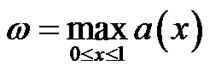 . By taking first terms of the Taylor’s series expansion for a(x) and b(x) about the point “1”, (14) becomes,
 (15)
(15)
From (15) we have
 (16)
(16)
where, .
.
For the right layer, the special second order scheme corresponding to Equation (4b) [one can see [16]] is:
 (17)
(17)
with y(0) = a and y(1) = b.
We introduce a fitting factor  in the upwind scheme corresponding to Equation (17)
 (18)
(18)
Multiplying (18) by h and taking the limit as h ® 0; we get the value of the fitting factor:
 (19)
(19)
The equivalent three term recurrence relation of Equation (10) is given by:
 ;
; (20)
(20)
where,
This gives us the tri diagonal system which can be solved easily by Thomas Algorithm
4. Numerical Examples
To demonstrate the applicability of the method, we considered five numerical experiments (two problems with left-end, one with right-end boundary layer and two non-linear problems). We presented the absolute maximum error compared to the exact solution of the problems. For the examples not having the exact solution, the absolute maximum error is calculated using the double mesh principle.
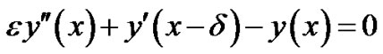
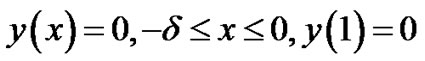
Example 1: Consider a singularly perturbed delay differential equation with left layer:
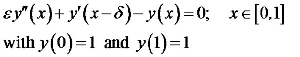
The exact solution is given by:

where,

The absolute maximum errors are given in Tables 1(a), (b) for d = 0.1*e and d = 0.5*e respectively.
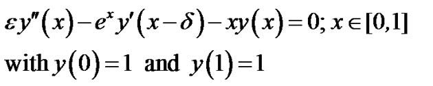
Example 2: Now we consider an example of variable coefficient singularly perturbed delay differential equation with left layer:


Table 1. (a) Absolute maximum error for Example 1 with δ = 0.1*ε; (b) Absolute maximum error for Example 1 with δ = 0.5*ε.

The absolute maximum errors are given in Tables 2(a), (b) for d = 0.1*e and d = 0.5*e respectively.
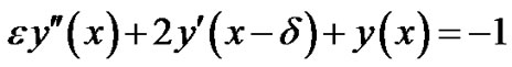
Example 3: Now we consider an example of variable coefficient singularly perturbed delay differential equation with right layer:
The absolute maximum errors are given in Tables 3(a), (b) for d = 0.1*e and d = 0.5*e respectively.
5. Nonlinear Examples
Here, the solution of the nonlinear singular perturbed delay differential problem is approximated by using the corresponding linear problem which is obtained by quasilinearization method.
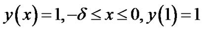
Example 4: Consider the nonlinear problem
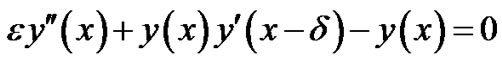
The linear form is:
 ;
;

The absolute maximum errors are given in Tables 4(a), (b) for d = 0.1*e and d = 0.5*e respectively.
Example 5: Consider the nonlinear problem

The linear form is:
 ;
;

The absolute maximum errors are given in Table 5(a) for d = 0.1*e.
6. Discussion and Conclusions
We presented an asymptotic-fitted approach to solve singularly perturbed delay differential equations of second order with left and right boundary. In this approach, the singularly perturbed delay differential equations is


Table 2. (a) Absolute maximum error for Example 2 with δ = 0.1*ε; (b) Absolute maximum error for Example 2 with δ = 0.5*ε.

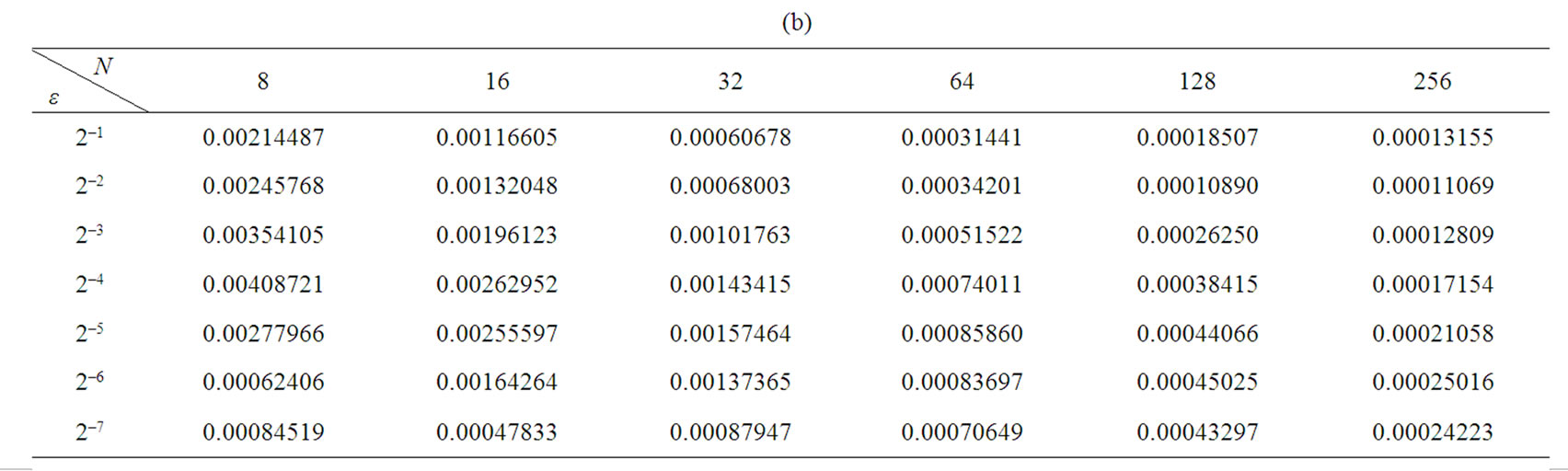
Table 3. (a) Absolute maximum error for Example 3 with δ = 0.1*ε; (b) Absolute maximum error for Example 3 with δ = 0.5*ε.

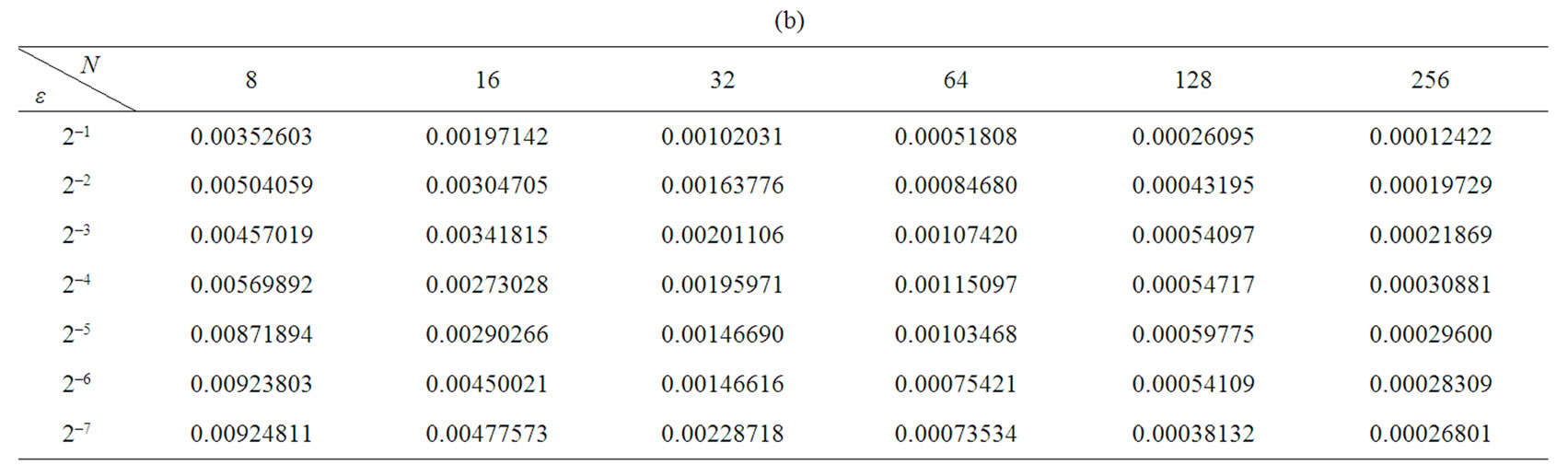
Table 4. (a) Absolute maximum error for Example 4 with δ = 0.1*ε; (b) Absolute maximum error for Example 4 with δ = 0.5*ε.

Table 5. Absolute maximum error for Example 5 with δ = 0.1*ε.
modified by approximating the term containing negative shift using Taylor series expansion. After approximating the coefficient of the second derivative of the new equation, we introduced a fitting parameter and determined its value using the theory of singular Perturbation; O’Malley [1]. The delay parameter ![]() was chosen so that the coefficient of the second derivative of the modified problem gets smaller. The final three term recurrence relation obtained is solved using Thomas algorithm.
was chosen so that the coefficient of the second derivative of the modified problem gets smaller. The final three term recurrence relation obtained is solved using Thomas algorithm.
Five problems were considered ((three linear problems; two on left layer and one on right layer) and (two nonlinear problems)) to test the applicability of the new method by taking different values of the delay parameter![]() , the perturbation parameter
, the perturbation parameter ![]() with the relation
with the relation  and
and  and different mesh size h. It is observed that the method produces good approximation for relatively large mesh size and as mesh size decrease from
  the absolute maximum error decreases. It is observed that this method is not producing good results for very small step mesh (h).
REFERENCES
- R. E. O’Malley, “Introduction to Singular Perturbations,” Academic Press, New York, 1974.
- R. N. Rao and P. Pramod Chakravarthy, “A Fourth Order Finite Difference Method for Singularly Perturbed Differential-Difference Equations,” American Journal of Computational and Applied Mathematics, Vol. 1, No. 1, 2011, pp. 5-10.
- H. S. Prasad and Y. N. Reddy, “Numerical Solution of Singularly Perturbed Differential-Difference Equations with Small Shifts of Mixed Type by Differential Quadrature Method,” American Journal of Computational and Applied Mathematics, Vol. 2, No. 1, 2012, pp. 46-52.
- M. K. Kadalbajoo and K. K. Sharma, “Numerical Analysis of Singularly Perturbed Delay Differential Equations with Layer Behavior,” Applied Mathematics and Computation, Vol. 157, No. 1, 2004, pp. 11-28. doi:10.1016/j.amc.2003.06.012
- M. K. Kadalbajoo and V. P. Ramesh, “Hybrid Method for Numerical Solution of Singularly Perturbed Delay Differential Equations,” Applied Mathematics and Computation, Vol. 187, No. 2, 2007, pp. 797-814. doi:10.1016/j.amc.2006.08.159
- M. K. Kadalbajoo and K. K. Sharma, “Numerical Method Based on Finite Difference for Boundary Value Problems for Singularly Perturbed Delay Differential Equations,” Applied Mathematics and Computation, Vol. 197, No. 2, 2008, pp. 692-707. doi:10.1016/j.amc.2007.08.089
- M. K. Kadalbajoo and D. Kumar, “Fitted Mesh B-Spline Collocation Method for Singularly Perturbed DifferentialDifference Equations with Small Delay,” Applied Mathematics and Computation, Vol. 204, No. 1, 2008, pp. 90- 98. doi:10.1016/j.amc.2008.05.140
- M. K. Kadalbajoo and D. Kumar, “Computational Method for Singularly Perturbed Nonlinear Differential-Difference Equations with Small Shift,” Applied Mathematical Modeling, Vol. 34, No. 9, 2010, pp. 2584-2596. doi:10.1016/j.apm.2009.11.021
- A. Bellen and M. Zennaro, “Numerical Methods for Delay Differential Equations,” Oxford University Press, Oxford, 2003. doi:10.1093/acprof:oso/9780198506546.001.0001
- R. D. Driver, “Ordinary and Delay Differential Equations,” Springer-Verlag, New York, 1977. doi:10.1007/978-1-4684-9467-9
- R. E. Bellman and K. L. Cooke, “Differential-Difference Equations,” Academy Press, New York, 1963.
- L. E. El’sgol’ts, “Qualitative Methods in Mathematical Analyses, Translations of Mathematical Monographs 12,” American Mathematical Society, Providence, 1964.
- C. G. Lange and R. M. Miura, “Singular Perturbation Analysis of Boundary Value Problems for Differential Difference Equations, V. Small Shifts with Layer Behavior,” SIAM Journal on Applied Mathematics, Vol. 54, No. 1, 1994, pp. 249-272. doi:10.1137/S0036139992228120
- C. G. Lange and R. M. Miura, “Singular Perturbation Analysis of Boundary Value Problems for differential difference equations, (VI). Small Shifts with Rapid Oscillations,” SIAM Journal on Applied Mathematics, Vol. 54, No. 1, 1994, pp. 273-283. doi:10.1137/S0036139992228119
- C. G. Lange and R. M. Miura, “Singular Perturbation Analysis of Boundary Value Problems for Differential Difference Equations,” SIAM Journal on Applied Mathematics, Vol. 45, No. 5, 1985, pp. 687-707. doi:10.1137/0145041
- A. Andargie and Y. N. Reddy, “An Exponentially Fitted Special Second-Order Finite Difference Method for Solving Singular Perturbation Problems,” Applied Mathematics and Computation, Vol. 190, No. 2, 2007, pp. 1767-1782. doi:10.1016/j.amc.2007.02.051
- E. Angel and R. Bellman, “Dynamic Programming and partial Differential Equations,” Academic Press, New York, 1972.
NOTES
*Corresponding author.