ABSTRACT

As the World built, time established. Economists, however, put the “time” in the “ceteris paribus” basket, i.e. outside demand, supply and price. Moreover, Newton was mistaken in assuming that time flows independently. We saw that since the establishment of analysis, one science borrowed from the other, and economics borrowed from Physics: equilibrium, continuity―where nature does not make leaps―as well as Adam Smith’s invisible hand; in addition, management borrowed negative feedback from mechanical engineering; Newton, unwillingly, however, made harm to management by giving ground to managers to consider “humans as machines”. A whole array of theories and concepts-mentioned-followed from this. But our research passed from surprise to surprise: time in finance has 3 types: clock, trading (investors) and fractal (fractions). Given the difficult concept of “fractality”, we gave a mathematical and a simple geometrical exposition. Moreover, time… in time series is distinguished in further 3 types: random (white noise), persistent (black noise) and antipersistent (pink noise). So far 8 types of time… Einstein added another one: time as the 4^th dimension of the Universe… Mathematics in its role in presenting reality-par excellence expressed by “Marginalism” in 1870 in economics―and by using the 1938 “logistic equation” (re-discovered in 1971)―we saw what a “control coefficient” changing in time can achieve by leading the system from stability to chaos. Equilibrium is only a special case when the degree of chaos is low. Economists (Hicks, Joan Robinson) attributed to equilibrium subjective interpretations; we agree that equilibrium is not technical, mathematical or belonging to markets, but psychological. Be happy when accepting a price to be in equilibrium with seller. Samuelson, before modern theory of chaos (after 1968) appeared, he dethroned equilibrium and proved that equilibrium is when firms “maximize profits”. Poincare H was the first to see “chaos” in 1889 and Samuelson P saw “nonlinearity” in 1947. Chaos revolution, however, re-enthroned time. Smale (1961)―a chaos pioneer, who proved the existence of chaos, argued that chaos is a characteristic of dynamics and dynamics is the time evolution of a set of nature’s (and economy’s) states (words in italics added). We applied the following 3 models: {1} $X_{next}=aX\left(1-X\right)$ ; {2a} $X_{n+1}=1-a{X}_n^2+Y_n$ and {2b} $Y_n{}_{+1}=b{X}_n$ and {3a} $\text{d}X/\text{d}t=10\left(Y-X\right)$ , (3b) $\text{d}Y/\text{d}t=-XZ+28X-Y$ and {3c} $\text{d}Z/\text{d}t=X^2-8/3Z$ . All models lead to chaos and all models embody time as consisting of difference or differential equations. These now are our tools if time returns into our analysis.

Keywords:

Time, Equilibrium, Maximization of Profits, Chaos Theory and Complexity, 3 Dynamic Models Applied to Shipping Markets

1. Introduction

As God built the world, the concept of calendar time established. The World built in 7 days (one week). During the “day” Sun is present, and during “night” Moon (earth’s satellite) shines. Also, 4 seasons are established by Earth approaching Sun at 4 different distances in 12 Moon rounds (336 days―a year). A month is also introduced by a complete orbit of Moon round the Earth (28 days).

1.1. Time in Economics

Economists do not display time during the determination of price by supply and demand, which are Marshall’s blades of a pair of scissors. Economists work their analyses under the assumption of “ceteris paribus¹” (Latin). Time is locked-in in ceteris paribus.

1.2. Time in Physics and Thermodynamics

Newton (1642-1727) thought time to be reversible. Thermodynamics, however, proved that time is irreversible… By mixing 2 fluids, e.g., red and blue, one gets purple; here the “entropy” is high, and “uncertainty”, related to it, is also high; these are time-dependent, and un-mixing is impossible. Moreover, the “molecular structure of universe” can only be described by probabilities…

1.3. Equilibrium in Economics

The condition of equilibrium economists tried―unsuccessfully, we reckon―to accommodate into economic analysis. Adam Smith (1723-1790) believed that selfishness provides a powerful fuel in a commercial society, a prior idea of “workable competition”; private interests are harmonized with social interests by an “invisible hand”. Obviously, Smith conceived a model of competition, not as it works, but how it should work―given also his engagement with his “theory of moral sentiments”, though no reference was made to this.

1.4. The Influence of Newton and Descartes

Most sciences and economics―as well management―were heavily influenced by the scientific principles of Newton and Descartes (1596-1650). They argued that the “natural state of a system” is the equilibrium, and departure from it will be damped out. Economists by adopting the concept of equilibrium were astonished by the two depressions in Black Monday and Tuesday (1929 and 2008).

In traditional management (1911-1947), equilibrium was a core principle! Fayol H (in 1916 in French; 1949 in English) and other early management writers (Taylor F in 1911) invented management control mechanisms based on the perception: “firms as machines²”, meaning “humans as machines”. Moreover, Weber M. (1946 in English) conceived “firms as bureaus”. Firms―as a result―functioned by drafting plans (planning), budgets and applying “management by objectives” (1965). This considered being a “command and control” system, where control is done through “monetary rewards” and “punishments”.

Moreover, “reductionism” (i.e. making complex matters less complex), introduced the systems: division of labor, “task”, standardized procedures, quality control (1991), cost accounting, and organizational charts. Also, the budget―used in shipping companies par excellence―performance reviews, audits, standards, etc. all applied controls. In fact, the negative feedback used i.e. a mechanism for maintaining a desirable equilibrium… No body, however, proved so far the benefits of equilibrium in management acting in a volatile world…

The classical system sought-out for amore “certain” reality. This was promised by the “command and control” pattern and this is what managers prefer on the basis of the principle: “achieve most with a minimum effort”. But everybody witnessed that business world became more complex-day after day (especially by Citibank and Xerox). Complexity increases over time, and in the case of living systems, like economy, this is called evolution. Some suggest correctly to absorb complexity instead of trying to reduce it.

1.5. The Necessity of Equilibrium

Do we need equilibrium? Yes, if we believe in determinism, predictability and balance. No, if we believe in structure, pattern, self-organization, life cycle (ideas from biology). Yes, if we believe that there is a single accessible end-point of balance. No, if external effects and differences are key-drivers; no, if any economic system is constantly “unfolding”. Yes, if there are no real dynamics and everything is in equilibrium. No, if economy is constantly on the edge of time; it rushes forward, structures constantly coalescing, decaying, and changing…

2. Aim and Organization of Paper

The purposes of this paper is: (1) to show the role that time plays in Economics, Finance, Chaos Theory, Physics and Shipping; (2) to state what exactly equilibrium means in Economics, Physics, and Complexity Theory; (3) to use the “logistic equation”, the Henon’s and Lorenz’s attractors in applying chaos to shipping markets and (4) to show the relationship between equilibrium and profit maximization due to Samuelson.

The paper is organized as follows: next is a literature review followed by methodology; then time in maritime economy and finance is presented. Next, the equilibrium concept in economics, Physics and Complexity Theory is showed. Then chaos theory is applied to shipping markets; finally we conclude. In Appendix we deal especially with the concept of time in Physics.

3. Literature Review

3.1. Time in Marshall

Time³ preoccupied Marshall ((1920) [1] pp. 92; 274; 287), whose “time” is characterized as “operational”, i.e. near the “clock” time. Blaug (1997 [2] p. 354) argued correctly that time “periods” in Marshall are short or long, according to the “partial or complete” adaptation of producers and consumers to changing circumstances. The actual clock-time periods in Marshall, however, left undefined. A matter which is very important⁴, especially when one wishes to pass from theory to reality. Moreover, in the preface of the 8^th edition of his book ( [1] (preface, pp. xii-xii)), Marshall was apologetic about the largely static character of his analysis with the frequent use of the “ceteris paribus” assumption.

3.2. Does Nature Jump⁵?

Marshall [1] believed that nature is smooth: “Nature makes no jumps” (leaps) (“Natura non facit saltum”) he stated, based on “principle of continuity” (Blaug (1997) [2] p. 379), an idea from Physics.⁶ However, unlike rivers, markets… jump (Mandelbrot and Hudson, (2006) [4] p. 85-86; 227-229)! Heraclitus (~460 BC) “said”⁷ that “one cannot enter into a river and encounter the same waters”, meaning that “everything is constantly changing”… in a process of “becoming”; something resembling emergence in the complex adaptive systems (Battram, (1998) [5] p. 13).

3.3. Marshall and Biology

Marshall ( [1] p. xii) argued that important for economics⁸ is “economic biology⁹ “... What Marshall meant―we believe―is that economy has to be studied at best as a living “organism’” (Blaug [2] p. 404) (italics added)). “Economic biology” means to introduce “continuous or discrete changes” into economic analysis. A “dynamic system” has the time as independent variable and a small number of dependent variables, the movement of which is controlled by rules. Time may be continuous (+∞ to −∞), a case where differential equations are used, or discrete, like in time series, a case where difference equations are used.

3.4. Hicks’ Economic Expectations

Hicks (1946) [6] , p. 120) argued that Marshall refers to a (final) supply for sale, determined by past expectations (taking into account preferences and incomes). Traders do not know what exactly suppliers will bring, or what buyers will demand. Prices thus are fixed by trial and error. Marshall argued that supply and demand must be equal: the buyers to buy what they desire (at the market price) and sellers to sell what they desire. Thus, equilibrium is a balance of desires… Hicks rejected the “full foresight” assumption, which Joan Robinson (1965; [7] ) restored by a new concept that of “lucidity”. Hicks (p. 140) said: “economists have often toyed with the idea of a system where all trading persons have ‘perfect foresight’―leading to awkward logical difficulties…”

3.5. Robinson’s “Lucidity” and “Tranquility”

Joan Robinson (1965) [7] ) argued indirectly that equilibrium (pp. 57-59), as a balance, comes from “celestial mechanics”, and it has to be applied with great caution in the “economics (of a stationary state)”. This metaphor is treacherous, she argued. Robinson transferred the concept of equilibrium from markets to people, by inventing 2 terms: tranquility and lucidity… Tranquility is when economy is in smooth regular markets… where expectations-based upon past experience―are very confidently held… constantly fulfilled and renewed over time, and lucidity, where people are fully aware of the situation in all markets etc.

3.6. Zannetos Applied Hicks’ Model in Tanker Shipping

Zannetos (1966; [8] ) adopted Hick’s theory of expectations ( [6] p. 117), where the current supply of a good depends mainly on the price that firms expected to be. This implies that if current prices are high, then future prices are expected to be higher, and vice versa. Zannetos (p. 239) argued that static economic analysis was unable to explain how rates were formed in tanker markets. There are substantial price movements―away from equilibrium―creating expectations that future rates will increase at a higher speed than hitherto. So, short term (spot) rates are formed by demand, as a function of “price expectations” and static supply (Graphic 1).

As shown, a number of partial equilibria are possible―outside R_s―the region of strict static relevance (and inelastic). E.g. the slopes of demand and supply in regions R₂ and R₃ do matter; supply has a negative slope. R₃ is stable from below and R₂ indicates a price in an unstable range, as demand’s slope is positive. R₄ shows potential instability. Prices could be at rest―given able time―at either R_s or R₃, but not at unstable R₂. Markets are prone to excess capacity and depressions.

Zannetos further argues (op. cit., [8] p. 21) that it is not unreasonable to assume that expectations alternate between elasticity and inelasticity, if the market stays long enough at an equilibrium point, before it goes into a spin…; as the memory of those operating in the market may not last long enough to recall how the market came at rest...

He applied the nonlinear model of “cobweb theorem”, where he found its adjustment paths to be similar with those of spot tanker rates in a plethora of webs. The fluctuations have the static long run equilibrium as a central focus (p. 244) (unstable). An empirical investigation using a questionnaire among shipping tanker companies is required, we believe, to confirm Zannetos’ theory today.

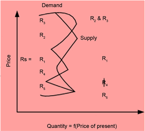
Source: modified from Zannetos (1966, [8] p. 18).

Graphic 1. Demand and Supply affected by price-elastic expectations determining freight rates a la Zannetos-Multiple equilibria a la Marshall.

Samuelson (Nobel winner) spoke with the language of Mathematics. Samuelson (1967) [9] ) re-published his “Foundations of Economic Analysis” on his ideas since 1947. Samuelson argued that economics is a softer, and less exact, science than conventional Physics (preface ix) and for Marshall, stability of equilibrium requires that the supply curve cuts the demand curve from below (p. 18 [9] ).

The idea of equilibrium¹⁰ Samuelson (p. 21) said is a matter of the equations involved in maximizing (minimizing) conditions. “All economic results emerge from maximizing assumptions” he argued (p. 22). Important are the slopes of the curves at equilibrium. Statical is the equilibrium of the intersection of a pair of curves (=Marshall’s case), which it may be stationary, and timeless, but holding over time (p. 313).

Samuelson devoted 8 chapters to analyzing comparative-statics. In 3 chapters, he introduced the “correspondence principle” relating comparative statics with dynamics (& stability). The last 2 chapters devoted to “dynamical systems” (also to stability etc.). He argued (p. 351) that Walras (1834-1910) provided the notion of the “determinateness of equilibrium” on a statical level, which Pareto (1848-1923) further elaborated. Pareto, however, laid the basis for a theory of comparative-statics, pioneered by Cournot¹¹ (1801-1877). Pareto failed to use the secondary conditions for maxima. Samuelson suggested “comparative-dynamics” (p. 351-2). A system is dynamical if its behavior over time is determined by functional equations in which “variables at different points of time” are involved in an “essential” way (p. 314) (the term “essential” comes from econometrics¹²).

3.7. Chaos Theory and Complexity

Nonlinearity opened a door nearer to reality. Samuelson (1967) [9] , p. 338) was aware by saying “linear systems lack the qualitative richness of nonlinear systems”, which “introduce also a theory about fluctuations”. He mentioned¹³ Birkhoff¹⁴ G D. He argued that (p. 339) in the field of economics only one nonlinear system received complete treatment: the “cobweb” theorem, in which supply lags and equals a nonlinear difference equation of the 1^st order¹⁵.

West and Goldberger (1987) [10] ) argued that the “physical fractal¹⁶ structures” are the ones generated by nature. They are more error-tolerant and more stable. One market can absorb shocks as long as it retains its fractal structure. Peters (1994) [11] p. 8) recognized that a 4σ change in time series is a crash (Goulielmos, (2017) [12] ). When market’s investment horizon shortens, the market becomes erratic and unstable. Do the real world and markets show local randomness and global determinism (Peters, (1994) [11] pp. 10-11)? Farmer and Lo (1996) [13] ) advanced a theory dealing with the “adaptive markets hypothesis”.

Abraham (2000) ( [14] p. 81-90) argued that Chaos revolution, 1968-1998, begun with the work of “Takens and Ruele” on “turbulence” ( [15] 1971)―mentioned also by Goulielmos (2017)―consisting the turning point in Science. To this “Thom” contributed (1973 [16] ) as well “Li and Yorke” (1975 [17] ), who brought the word of “chaos” out.

Chaos, however, glanced first by Poincare H. in 1889. Poincare participated in a mathematical competition, set by King Oskar II of “Sweden and Norway”, for the participants to solve a problem¹⁷. In solving it both Prof. Weirestrass and Poincare-in his 1st attempt-failed. Poincare, as a result of the competition, and due to a mistake he made, discovered accidentally the “homoclinic tangle” or Chaos (Graphic 2), as shown in his paper published in 1890 (by which he won the competition). The case of ∞ solutions of the above problem is indeed related to “homoclinic” behavior (Smale¹⁸ [18] ). A “homoclinic tangle” is found in the manifolds of certain maps (Harding¹⁹ (unknown date)), if manifolds cross transversally.

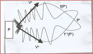
Source: inspired by Harding (unknown date).

Graphic 2. Let P be a fixed point saddle; then p' is a homoclinic point. f(p') and f⁻¹(p') on stable and unstable manifolds are also homoclinic points, as nà∞.

Smale (2000) [18] (p. 20-21) proved that if a dynamical system possesses a “homoclinic” point then it also contains a “horseshoe”. Time is considered by Smale as a continuous entity, but measured by discrete units. He said that chaos is a characteristic of dynamics, and dynamics is the time evolution of a set of Nature’s states ( [18] p. 13).

Farmer (2002) [19] ) supported the idea of biology in economics-arguing that… “market ecology” shows how financial firms engage in specialized strategies, which can be sorted into groups analogous to species in biology. Kirman (1997) [20] argued that the very process of learning and adaptation and the feedback from the consequences of that adaptation generate highly complicated dynamics, which may well not converge to equilibrium…

Stopford (2009 [21] , pp. 163-168), in shipping economics, copied Marshall in his analysis of the 3 periods: market, short run and long run, though Marshall had and a fourth period: the “very long run”, ignored by Stopford, but not by Goulielmos (2017 [22] ).

In summary, Marshall introduced time in the form of 4 periods into economic analysis, as a method of exposition, but with a recreation and tool to reality. Moreover, another unreal assumption of Marshall, and not only, was “ceteris paribus”. Finally, while Marshall was “flirting” with dynamics, it was²⁰ Samuelson to write about. Hicks transferred the concept of equilibrium from price formation to human expectations. Hicks removed also one leg from the model of Perfect Competition that of “Perfect Foresight”. Joan Robinson kept distances from equilibrium and instead introduced the concepts of “lucidity” (for foresight) and “tranquility” (for equilibrium).

Economics waited Samuelson [9] to upgrade its status by expressing most of it in mathematics: a recreation and tool’... he wrote (p. vii). Samuelson (1967) [9] dethroned equilibrium as the prime end of enterprises (microeconomics) and replaced it with the “maximization of profits”. He cleared out concepts like statical²¹, comparative-statics, comparative-dynamics, dynamics²² etc. He established the “intimate formal dependence between comparative-statics and dynamics”. Moreover, Samuelson classified dynamics in 6 different classes…

4. Methodology

The “logistic equation” {1} will be used here to simulate equilibrium in shipping markets: X_next = aX(1 − X) {1}²³. Important is coefficient “a” or C (0 - 4): a parameter describing the characteristics of the system; X_next is a variable (0 - 1, or 0% - 100%) in future (%), 1 − X gives what remains of X over time and X₀ = the initial rate (assumed 50% or 0.5).

We must mention that Ruelle²⁴ D. [23] supported mathematically the existence of “attractors”²⁵―to be used below-showing the behavior of natural systems; the tendency of a system is to move toward some underlying pattern (as energy is lost). We will use two well-known attractors―“Henon’s” and “Lorenz’s”―which we will apply to find out equilibrium in shipping markets.

5. Time in Maritime Economy

Time in Physics is presented in Appendix. In Figure 1, the freight rate determination appears in shipping industry and the firm (=vessel), by supply and demand, but with time absent...

The above is a “photograph”. It is taken of a freight market on a certain date and time; a static picture… of a dynamic market. Alternatively, maritime economists applied the so called “comparative-statics” by allowing shifts in the curves caused by changes assumed to occur in the factors presented-like supply of ship space. This moved to the right (3 shifts, Figure 1, left part).

The time needed for shifts to occur and their extent, are not shown (shifts assumed here are equal, parallel, and positive). “Comparative-statics” determine only the direction in which variables change, as a result of a disturbance to original equilibrium (F₁). Only the new equilibria (F₂, F₃) are shown, which can be “compared” with the previous one F₁. This is a comparison of two photographs taken at different times.

Figure 2 is the only graph in shipping economics―to the best of our knowledge―where time is included in the freight rate determination (Shimojo (1979) [24] ); McConville, (1999) [25] , pp. 253-4).

As shown, time affects freight rates, because the 3 supply and the 3 demand curves differ at the 3 times: T, T₁ and T₂, where F₁ < F < F₂ and Q < Q₁ < Q₂. If equilibrium is affected by time, why maritime economists put it out in ceteris paribus?

6. Time in Finance

In finance exist 3 times...: “Clock”, “Trading”, and “Fractal” (Mandelbrot and Hudson (2006; [4] p. 22), (Figure 3).

6.1. Clock Time

The clock time is linear; this is in which we think.

6.2. Trading Time or θ-Theta

Trading time is the time in which markets operate; investors’ time. Θ is a random non-decreasing function of clock time; an intuitive notion of how markets operate over time (Mandelbrot (2010) [26] p. 163)). Both θ(t) and X(θ) are “self-affine” functions, i.e. similar under different scales. Θ intervenes in linear clock: it speeds-it-up in periods of high volatility and lows-it-down in periods of

stability. Market scales²⁶. Economics have no intrinsic time scales. Θ is flexible.

Another kind of clock is needed to measure θ… The actual implementation of Θ generalizes the generating equation: y^1/H + (2y − 1)^1/H + y^1/H = 1 {1}. The root of this equation, H, when determined, it can define the 3 quantities above in {1}: Δ₁θ, Δ₂θ, Δ₃θ, which all add to 1. Θ as a function of clock time no longer reduces identically to clock time (Mandelbrot, (2002), [27] p. 76-77)). Let Δx be the order of a magnitude of a “price change” over a time increment Δt (small): then, Δx ~ Δt^1/α or Δx ~ Δt^H, where 1/α = H: time invariant (but ≠1/2); alpha is a power exponent and H is Hurst’s exponent. Then X(θ) stands for a price function of θ, and thus X[θ(t)] = P(t).

6.3. Fractal²⁷ Time-FT

FT is equal to θ, but only when ruled by “devil’s staircase”²⁸ (Mandelbrot (2010) [26] p. 41). FT does not influence the statistical characteristics of the object (or chart) under study (Peters, 1994, [11] p. 5). Self-similarity exists, meaning that the object or process in time is similar at different scales: spatial, temporal, statistical. A fractal is scale-invariant and it lacks a characteristic scale. This is a power law scaling too. The feature, which turns out to be the 2^nd characteristic of fractals, is dimension. A random walk has a fractal dimension of 2. A shipping freight rates index for dry cargoes since 1741 has a fractal dimension 1.30.

A fractal and multifractal model (following Farmer D. in 1980 and Mpountis T (2004) [30] p. 228)).

Let the number of high and low prices in a market [0 1] be N. Let the % of high prices be: p₁ = n₁/N, and of low prices-distributed in two groups-be: p₂ = n₂/N, where n₂ < n₁, so that: p₁ + 2p₂ = (n₁ + 2n₂)/N = 1 {1}. One histogram has 0p₁ peak-in the middle-and a base extending from 1/3 to 2/3, and 2 other histograms (left and right), which have a lower peak 0p₂, and a base extending from 0 to 1/3 for the left and from 2/3 to 1 for the right (Figure 5).

Each of the above 3 distributions are divided into 3 further distributions, the heights of which are multiplied by p₁, for high prices, and by p₂, for low, in n steps. The result is that low prices eventually become numerous. The group that plays the more serious role (high prices) can also be found, with probability: $P_{m1}^{\left(n\right)}$ as n à ∞, and m = m₁, where $N_{m1}^{\left(n\right)}{P}_{m1}^{\left(n\right)}$ , is at maximum as n à ∞. Skipping the proof²⁹, the final result is m₁ = 2p₂n.

²⁹Shown in Mpountis (2004) [30] p. 229 (in Greek).

Now, if p₁ = p₂ = 1/3 or p₁ = 0 and p₂ = 1/2, this is the simple fractal (of a single dimension). This (dimension) is given by: D₁ = p₁logp₁ + 2p₂logp₂/log(1/3) = 1 {2} if p₁ = p₂ = 1/3. And ~0.63, if p₁ = 0 and p₂ = 0.5. This indicates that dimensions are ∞, and this market is multifractal. D₁ can indeed be generalized for all real numbers q, denoted by D_q (not shown). Figure 4 shows the peaks of $P_1^3$ and $P_1^2{P}_1$ histograms of high prices and low ones. The graph is a mathematical fractal construction of histograms so similar to those of… an “actual” market!

6.4. Time… in Time Series

Another distinction of time is given below (Figure 5):

As shown, “time”… in time series can be: (1) random, (2) persistent and (3) anti-persistent. As argued by Peters (1994 [11] p. 5), most people support the idea that time is deterministic. But, we have random catastrophic events, like natural and economic disasters (Goulielmos, 2017 [12] )...

6.5. Time in Einstein (1905) [31]

This is: T = D² {1}, where D stands for distance covered by a random particle, and T stands for clock time used to measure it. Equation {1} can also be written as T = D^H {2}, and H = 1/2. Equation {2} is a generalization of {1} due to Hurst (1951) [32] , where H takes values in the interval [0 1] and D = Range. Time in logs is: log(T) = log(D) + log(c)/H {3}. Einstein added one further dimension in Universe: the 4^th dimension (=time).

Persistent time is T^H = D/c {4}, when c is a constant, T stands for time and 0.5 < H ≤ 1. Anti-persistent time is T^H = D/c {5}, when 0 ≤ H < 1/2.

Figure 6 shows the log of random time (red line) and the real time (blue line) at which the time series of the “Baltic Panamax Index”―“travelled” from 1999 to 2012. Figure 6 comes from: log(R/S) = log(kT^H) = log(k) + Hlog(T), where R is the range, S the local standard deviation, H is the power law, T = n = time index and k is a constant. Range is the difference between the maximum value of a time series from its minimum value.

As shown, the time series for “Baltic Panamax Index” (blue line) travels faster than random-covering more distance. So, time series is persistent (has a long memory or “black noise”). These time series have trends, and if a rise occurred in t − 1, the chances are that it will continue to increase in t + 1. However, they are subject to sudden falls and rises. They have runs of + values that persist for some time, before switching to negative runs, which also persist. The distance

travelled is proportional to a power of the time elapsed, the power taking any value between 0 and 1.

7. Economic Equilibrium

Marshallian ((1920) [1] pp. 286-288) equilibrium is the situation, where the “amount of a good supplied” equals the “quantity demanded”―at a certain price (called equilibrium). Before that, “supply price” has to be equal to “demand price”... = the Marshallian condition for equilibrium (Blaug (1997) [2] p. 388)³⁰. Attention is needed to the “demand” and the “supply” price: we reckon, that before buyers and sellers go to market, they pre-calculate their “prices”, including costs and “margins”³¹ (profits) at every quantity... Profit is also included in the “demand price” for buyers, and this is something different at each quantity bought (as costs differ). These profits, we believe, are the “forces in action”, to copy Physics, and also these are the independent variables…

7.1. How We Would Like to Interpret Marshall’s Analysis?

Let “supply price” Q_si (average) be: P_i = (TC_i + Π_i)/Q_i {1}, as a function of profit Π_i and of total costs of production TC_i, pertaining to quantity produced Q_i; where i is a time index, taking values from 1 to n. Moreover: profits Π₁ < Π₂ < Π₃, ・・・, < Π_n {2}, as an incentive to produce more, when prices P₁ < P₂ < P₃ < ・・・ < P_n {3}, and if Q_di > Q_si, and vice versa³², where Q_di is the quantity demanded at time i; n = 1 stands for start-up time.

We introduced falling costs, as production over time increases, resulting in increasing profits; this is―we reckon―a force for producers to produce more, when “asked” by buyers. Marshallian costs can be constant, increasing or falling. For buyers (merchants rather) Marshall makes no reference to their costs, but only to their (resale) profits.

As a result of the above analysis, a producer is in a pre-equilibrium in any quantity, given his/her “supply price” is paid by buyers. And buyers are in pre-equilibrium in any quantity, if their “demand price” is met. For the market, and for both―sellers and buyers―to be in equilibrium, “supply price” must be equal to “demand price”, at a common quantity: the equilibrium quantity. Buyers and sellers go to market prepared with accounting information to find-out there which price will be established.

7.2. Equilibrium with Curves

Figure 7 gives Marshall’s concept of equilibrium geometrically. Let 0R be the rate of production―actually taking place―and Rd the “demand price” and Rs the “supply price”. If Rd > Rs, production 0R is exceptionally profitable, and will increase, where R is the “amount index” (moving right or left). The reverse will happen if Rs > Rd. Equilibrium is achieved when Rd = Rs, and is stable with the shape of the curves shown.

7.3. The Laws of Demand and Supply

The movement along a demand or a supply curve, is based³³ on 2 “economic forces”: (1) when price increases, supply increases; and vice versa; and (2) when

price increases, demand falls; and vice versa. This shows that the move along the 2 curves is of the opposite direction, as shown by arrows (Figure 7). Thus, a crossing of the two curves will definitely occur at a certain price and quantity, i.e. the 2 curves will intersect = at the “equilibrium price” and “quantity”; these two forces give the desired stability. As a result, we must be careful that the laws of demand and supply are valid, when equilibrium is examined, something not always certain…

7.4. A Psychological Equilibrium

This³⁴ is a state when “expectations of the sellers meet the expectations of the buyers”. Is it possible for market players to realize their expectations? Yes. If the quantity brought into the market by sellers is all sold at the pre-determined profit. If the price asked from the merchants to buy their expected quantity at their profit is the same. This is equilibrium; this, however, can be achieved only by coincidence... or what Hicks said by trial and error. Here satisfaction in both sides is achieved, where no stocks are created and no demand goes away with empty hands…

7.5. The Stability of Equilibrium

What is not so convincing from the above analysis is that if Q_d < Q_s, price will fall, and if Q_d > Q_s, price will increase. Surely, if Q_d < Q_s, stocks will be created and producers will be unsatisfied. Will, however, producers lower their price to sell the entire amount, provided they have brought it to the market and their goods cannot be stored? If Q_d > Q_s, then producers must have a stock to sell. If there is no stock, then demand will be unsatisfied. It is possible then for the price to increase next time. Thus the whole idea that equilibrium will be achieved, even if disturbed, has to be re-examined, as much confusion has been created and hopes remained unfulfilled.

7.6. Equilibrium in Physics

In Physics (Young and Freedman (2000) [3] p. 97)), equilibrium is when a body is acted on by no force; and when a body acted on by several forces, where their vector sum is zero. This body is either at rest, or moving in a straight line, with a constant velocity. Economics has adopted the second, when demand (force) is cancelled by supply (force) and price and quantity are at rest. But can price and quantity also move―as they are―with constant velocity? Theoretically they can.

Equilibrium in Physics is based on Newton’s 1^st law, saying that a body acted on by no net force moves with constant velocity, or 0, and a zero acceleration ( [3] p. 96). So, economic “static” equilibrium will be attained, if the force of demand is exactly cancelled by the force of supply. How do we know that this is a static equilibrium? Because, price moves at zero speed. If we assume that price moves at constant speed―as Physics argued―is exactly what Hicks ((1946) [6] p. 132) said that “prices move constantly into future in a stationary equilibrium over time”.

7.7. Equilibrium versus Profit Maximization

Given that maximization of profits is the true end of firms, one may ask what is the connection between this end and “equilibrium”? Samuelson (1967, [9] p. 88) placed indeed “profit maximization” prior to “equilibrium”, as the former is indeed the 1^st fundamental assumption for him.

7.8. The Relationship between Equilibrium and Profit Maximization

Equilibrium needs production with factor combinations so that TC (total cost) is at minimum: the marginal productivity of the last $ is equal everywhere, and the price of each factor of production is proportional to its Physical productivity (marginal), in analogy to marginal cost; the output selected, maximizes net Revenue, and total cost is determined optimally: MC (marginal cost) = MR (marginal revenue)-with a smaller slope than that of MR; the value productivity of each factor (marginal) = its price (MR times marginal physical productivity); and TC ≤ TR.

7.9. Equilibrium in Complexity Theory

Battram ((1998) [5] p. 157 and afterwards)) argued that firms can be frequently locked-in to a less than optimal state (meaning < equilibrium). It is strange, but no one in management asks for whether a company achieved equilibrium...

8. Applying Chaos to Shipping Markets

8.1. The Laid-Up Tonnage as a “Logistic Equation”

Let laid-up³⁵ tonnage follow the quadratic equation³⁶: X = aX − aX² {1}, where X stands for laid-up tonnage and “a” is the control coefficient; X(a − aX − 1) = 0 {2}. One of its solution is X = 0, where no laid―up tonnage―LUT, exists; and another solution is X = a − 1/a. Both solutions are interesting. Equation {1} graphically is presented below (Figure 8).

At low levels of “a” there is stability and constancy; as “a” increases, emerge oscillations, complex patterns, disorder, and the whole system “appears” random. Let now take 20 time periods (Figure 9) using the iteration method (i.e. the solution X₁ at t₁ is inserted into X₂, and so on). At a = 80% (0.8), LUT declines continuously and stabilizes at X = 0. At a = 1.5, LUT = 33%. These cases are examples of low-order chaos, and are stable and predictable. At a = 3, LUT

oscillates between 63% and 70%. This pattern, between a = 1.5 and 3, gives the 1^st bifurcation. Then at higher a’s, LUT “exists” alternating between 88%, 37%, 83% and 51% (Figure 9).

In 1971, May³⁷ R. re-discovered equation {1}, which shows an inherent tendency of a simple nonlinear system to go through period doubling. If the solutions are constant (a = 1.5) or oscillating with regular, periodic solutions: a = 3 or 3.55, then they are more capable in re-establishing regularity after being drawn away from their regular pattern: this is stability.

Laid-up tonnage obeying the logistic equation gives 3 types of curves for t = 1 to t = 20 and for a = 0.80, 1.50 and 3.00. We assume also an initial tonnage in laid-up equal to 50% (0.50), as a starting condition. This means we start when market is in a deep depression, like in 1981-1987 (Graphic 3).

As shown at t = 5, 10 and 15 time periods 3 logistic equations appear-with 3 different a’s. The conventional Marshallian equilibrium is at t = 15, where S = D, and LUT (%) is zero. This is a “structurally” stable point. The amount (%) of LUT is continuously falling from an initial 50% to 20% and 0% over time. Shipowners are happy.

However, if Market gets worse, if “a” gets higher, the LUP tonnage increases to a (stable) 33% (a deep depression). Here a heavy effort due to extensive scrapping of ships could reduce LUT by 12%, but after 1 - 2 periods it will return back. At a higher “a” = 3.00, appears a stable and continuous oscillation ranging from 63% LUT to 70%, i.e. a heavy depression. Finally, the LUT alternates among: 88%, 37%, 83% and 51%, for every 4rth period, for a > 3.00 (not shown here), manifested is the well-known shipping cycle; “a” can get values from 1 to 4. At a = 3, this is the last time when market is in equilibrium; at a = 3.45 the period is doubling (X(aX − a) = 0) and at a ≥ 3.57, we enter chaos. Massive recent LUT is shown in Graphic 3.

The above model is only one-variable model. Of course laid-up tonnage reflects the final result of supply and demand.

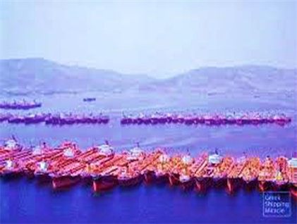
Source: Greek shipping world (unknown date).

Graphic 3. Laid-up tonnage for lack of demand in a recent Shipping depression.

8.2. Shipping Markets as an Attractor of 2 Difference Equations

Let assume now another model³⁸―with 2 difference equations: Supply for ship space = $X_{n+1}=1-a{X}_n^2+Y_n$ {1} and demand for ship space = Y_n+1 = bX_n {2}, where n = 0, 1, 2, ・・・ If $\left|b\right|$ < 1, X_n and Y_n are attracted by a set of points-as time (n) à ∞. The following graph (Figure 10) is derived if a = 1.4 and b = 0.3. When a > 0, and small, the attractor is quite simple.

To restrict the above model to have X ≥ 0 and Y ≥ 0, as demand and supply are positive, we excluded all negative values of X and Y (shaded part). We have introduced time (n). When Demand is at maximum, and Supply is zero, price is high. Thereafter, demand and supply move in balance, though dual amounts occur. Coefficients “b” and “a” stand for: “seaborne trade” and “shipbuilding prices” respectively. The supply of ship space is adaptive to demand as most maritime economists assume.

8.3. Shipping Markets in 3 Differential Equations

A more complicated dynamical model³⁹ with 3 differential equations is: dX/dt = 10(Y − X) {1}, dY/dt = −XZ + 28X − Y {2} and dZ/dt = XZ − 8/3Z {3}, Δt = 0.01, and initial conditions Xo = 6 = Yo and Zo = 27. Where X is the supply of ship space, Y is the demand for ship space and Z is the price or freight rate. In fact we have 4 variables including time. Attractor’s dimension is fractal and equal to 2.07.

As shown, Figure 11 depicts a system of 3 differential equations, which produce a “strange” attractor (right). Although we assume that the freight market is like weather, we have to put conditions so that none of the 3 variables as well time can take negative values. The model, however, does not provide an equilibrium as demand is higher than supply (left) at the intersection of the curves.

9. Conclusions

Economists locked in time in “ceteris paribus”, unable to work in a 3-dimensional space, where demand, supply, price and time could be presented. Marshall did not explain the content of ceteris paribus. Economic theory is mainly static. Economics made a progress by shifting the curves achieving the “comparative-statics”, thus obtaining 2 photographs at 2 different times to compare.

Reality obliged economists, and Marshall, to introduce 4 periods, where time is loosely and unrealistically defined: market period, short run, long run and very long run. Time is best represented by a differential equation.

While “marginalism” “saved” economists giving mathematics a prominent role in economics, after 1870, Marshall (in 1890) wrote that mathematics is scaffolding, which should be removed. Marshall innovated for placing price on Y axis and quantity on X for the first time.

One is surprised to find out that time has so many different expressions among sciences. Physics has one time for every area; maritime economics ignored time, but Japanese Shimojo; finance has 3 concepts for time, but “fractal” time is quite realistic followed by “trading” time. Chaos theory re-introduced time into economic analysis using differential and difference equations.

Equilibrium condition is adopted from Physics, appears nowhere in management, obscures the fact that maximization of profit is the true and unique end of enterprises. Enterprises are satisfied if they maximize their profits. Another obscure point is the belief that equilibrium―if disturbed, it returns to it―a hope that has been proved false crisis after crisis and at the end of 2008 meltdown par excellence. Equilibrium is a technical condition to say that what is demanded is

supplied, at a price securing the profits/utilities of both sides. Being in disequilibrium is more interesting.

Stability is a function of time. If we want a constancy, and stability, we need a low-level chaos adhering to a simple “attractor”. But no one excludes high-order chaos, which follows a more complex “attractor” with periodic oscillations.

Logistic equation is a well-celebrated tool applied here to represent laid-up tonnage. One is surprised to find out that laid-up can produce 4 different behaviors over time, where at a = 3 tonnage varies from 63% to 70%, and back to 63% in a continuous pattern. Similarly the model Demand = X_n+1 = 1 − aX_n + Y_n and Supply = Y_n+1 = bX_n, can determine the freight rate using 2 difference equations.

Finally, Demand and Supply determined price over time using 3 differential equations to describe shipping market like… weather. In dynamical systems, the state of the economy is represented by a set of variables and a system of difference equations, or differential equations, which describe how these variables change over time. Because new niches, new potentials, new possibilities, are continually created, the economy operates far from any optimum or global equilibrium. Systems are the adaptive nonlinear networks a la John Holland (in 1988).

Cite this paper

Goulielmos, A.M. (2018) Time and Equilibrium: 2 Important, But Invisible, Concepts of Economics, with Application to Shipping Industry. Modern Economy, 9, 536-561. https://doi.org/10.4236/me.2018.93035

References

Appendix. Time in Physics

Newton (in 1687) argued wrongly that “time flows equally without relation to anything external”. Let place a mirror in a box’s top and a light source at bottom (Figure A1). Box’s height = L. The light travels straight up the distance L at its speed c. At time $t^{\prime }$ = L/c {1}. We move mirror to right in a distance 1/2vt. The light travels up now by shortest distance⁴⁰: the hypotenuse. The Pythagorean theorem gives its length = [(1/2vt)² + L²] {2}. Light returns to its source through the other hypotenuse down, and thus the total distance is 2 times equation {2}. Raising {2} to square power and taking the square root, we have: [(1/4v²t² + L²)2] {3}, equal to ct.

Subtracting v²t² from both sides of {3}, divide by c² and take the square root of both sides, we get: $2L/c=t^{\prime }=t\sqrt{1-v^2/c^2}$ {4} (where v now is a fraction of c). Here, we have 2 times: t and $t^{\prime }$ ! Equation {4} states that time $t^{\prime }$ (between 2 events⁴¹ measured in a reference frame at the same place) = to time t (between 2 events measured in a reference frame at a different place), multiplied by the square root of 1 − v² ((where v is the (relative) speed of the 2 reference frames (as a % of light’s speed c)). So, time t between 2 events―at a different place―is greater of $t^{\prime }$ ―by $\sqrt{1-v^2}$ ―where $t^{\prime }$ is the time between the 2 events at the same place… Example: let v = 0.8⁴², then $t^{\prime }$ is 60% of t.

[*] Wolfson, R. (2003). Simply Einstein: Relativity Demystified, W W Norton & Co, NY, ISBN 0-393-05154-4.

NOTES

¹It means that all other (relevant) factors, with the exception of those presented in stasis, are constant. This expression means in English: “other things being equal”.

²This is a theory derived from “Control theory” and “Cybernetics”―systems dynamics. The idea was to reduce variety.

³Except the “time preference” issue.

⁴In shipping, “short run” is defined as the period when a company cannot change its capital: capital in shipping consists of…the “number of ships”. But to sell or buy a used ship is a matter of 1-3 months. This “long” run is really… very short in actual time. To build a ship is surely a matter may be of even 2 years on average. This is really “long run”... So, long run has 2 different durations, depending on whether we use new or used capital…Also firm’s long run with used capital is different than industry’s long run with new capital… Moreover, growth is not realized if industries use used capital…, but this is growth for an individual firm...

⁵Samuelson P. A. (1970) The fundamental approximation theorem of portfolio analysis in terms of means, variance and higher moments, Review of Economic Studies, 37, 537-542.

⁶The mass of a fluid is the same. If a water pipe―with a diameter 2 cm―is connected with a pipe of 1 cm―the flow speed of the fluid―not compressible―will be 4 times higher. The speed of the flow of a moving fluid is changing (Young and Freedman, (2000) [3] p. 439)).

⁷Kratylos, pupil of Plato, said: “Heraclitus argued that everything moves, and nothing is immobile, and humans―in front of the flow of a river―cannot enter twice in the same river” (waters). Aetios said that Heraclitus dismissed the state of rest and of immobility from everything, and everyone, as this is a characteristic of the dead. He attached to all a movement: eternal to eternals and temporary to temporaries. See: Heraclitus―all his work―collected by T Falkos-Arvanitakis, Zitros editions, 1999, ISBN 960-7760-36-0 (in Greek).

⁸A “dynamic economic system” has a set of variables―acting one on another―evolving in time, and following certain specific laws or rules.

⁹“Economic biology” is a study of scientific “laws” ruling an economy. “Economic ecology” studies the way economic agents are related one to the other and influenced from, and affect, their economic environment. Ecology is a branch of biology. Economics borrowed from ecology the idea that firms are living organisms.

¹⁰In a simple Demand and Supply model, price p and quantity q are the unknowns and equilibrium is: q − D(p, a) = 0 and q − S(p) = 0, where “a” is a shift parameter (e.g. for tastes), and where Dp < 0 and Da > 0 (p. 260).

¹¹Founder of mathematical Economics.

¹²Ragnar Frisch, On the notion of equilibrium and disequilibrium, Review of Economic Studies, III (1935-36), 100-106.

¹³Cartwright M and Littlewood J L, during World War II, proved mathematically that signs of chaos could exist.

¹⁴The ideas of Poincare (Jules Henri, 1854-1912, from France, Prof. of Mathematics in Paris) continued in USA by the American mathematician Birkhoff G D (in 1927; and in 1968)―a Professor at Harvard. But this movement died-out; lived in Russia, Berlin and Holland. In USA Lefshetz S revived the “dynamical systems theory”. Samuelson mentioned also Van der Pol (in 1926), Levinson N (in 1942; in 1944)―an MIT mathematician, Smith (in 1942) and Karman (in 1940); he was aware also of Mandelbrot.

¹⁵Zannetos [8] applied this model to tanker economics (p. 188-201; 243-4), as mentioned.

¹⁶Fractal is―broadly speaking―a new branch of Mathematics and of Geometry, which appeared in 1982 in English, used first… by God, who unlike Euclid, used fractions. This mathematics can be found in all natural constructions and in the human body.

¹⁷The problem: “Take a system of an arbitrary number of point-masses in gravity (according to Law of Newton), but not colliding”: “find the equation of the coordinates of each point as a function of time”. Smale solved it in 1961, 72 years later.

¹⁸Smale S. wrote a thesis in topology―1956―and proved the Poincare Conjecture for all dimensions > 4 in his “Generalized Poincare’s conjecture in dimensions > 4, Annals of Mathematics, II series, 74, 2, 391-406, 1961. In 1967 he also published: “Differentiable Dynamic systems”, Bulletin of the American Mathematical Society, 73, 6, p. 747-817.

¹⁹See his “The Homoclinic Tangle and Smale’s Horseshoe Map” in [14] .

²⁰Samuelson argued (p. 311, fn. [9] ) that in none of his writings Marshall showed more than a passing familiarity…with the biological notions of his time. Marshall influenced by Spencer H, (1820-1903), an English philosopher, who was after the unification of all knowledge on the basis of the single principle of evolution (1860).

²¹It refers to the form and structure of the postulated laws determining the behavior of a system (equilibrium). This is how stationary state is defined.

²²Defined by difference equations; and differential ones of course.

²³Due to Belgian mathematician Verhulst P F (1804-1849), who called it “logistic function” (1938): $X_{n+1}=a{X}_n-a{X}_n^2$ , as a reaction to Malthus T R (1766-1834), who argued that population grows at $N_{\left(n\right)}=N_o{a}^n$ (Malthus: “Essay on the principle of population”). See also Michailides T and Mpountis T, (2017), “Talking to Athina about Chaos and Complexity”, in Greek, ISBN 978-960-16-7778-1, Pataki editions, Athens. Samuelson ((1967) [9] p. 291-294) mentioned “logistic law”―i.e. the nonlinear difference equation: $\text{d}x/\text{d}t=x\left(1-x\right)$ or $\text{d}x/\text{d}t=x-x^2$ .

²⁴Belgian physicist―Prof. of Theoretical Physics at the “Institut des Hautes Etudes Scientifiques” near Paris―one of the founders of Chaos theory.

²⁵In the long term, a general dynamic system is adapted to attractor. The attractor “attracts” the system asymptotically. An attractor is part of its “phase space”―a mathematical space―such that a point from a near position approaches―as time goes-by―increasingly. See Ian Stewart, (1989), Does God play Dice? The new mathematics of chaos, B Blackwell, p. 132, in Greek translation (1998), ISBN 960-7122-01-1.

²⁶Moreover, each time-scale, each holding-period, for a stock or a bond, has its own risk. Price variations scale with time.

²⁷The term “fractal” comes from the Latin verb “frangere”, meaning to break something; it has been introduced in 1975 by B Mandelbrot in French: “Fractal Geometry of Nature”. In fact this means to deal with fractions.

²⁸The dependence ρ(Ω) is devil’s staircase, where each rational ρ = p/q, is represented by an interval of Ω values (the p/q-locking intervals). If r = 0, then ρ = Ω, where ρ is a rotation number. Αcircle map is Xt + 1 = f(Xt) or Xt + Ω ? r/2πsin(2πΧt), which is a transformation of the phase of one oscillator through a period of the 2^nd one. Ω describes the ratio of undistributed frequencies and r governs the strength of the nonlinear interaction [28] [29] .

²⁹Shown in Mpountis (2004) [30] p. 229 (in Greek).

³⁰The concept of “maximization of profits” is not mentioned at this stage…

³¹Marshall refers to the “gross earnings of management”.

³²This implies decreasing costs of scale; lower costs due to learning; time to advertise; economies of scale; reputation etc.

³³The “laws” may not work. Suppose one consumer―because of Christmas―stockpiled Coca Cola for 20 days; soon after Christmas, there is a special offer at reduced price; obviously no sale is expected to take place by the consumer (Priesmeyer (1992) [26] pp. 70-73). Thus, price falls, but quantity demanded does not rise.

³⁴After having written this, I read Hicks (1946) [6] saying: “the degree of disequilibrium marks the extent to which expectations are cheated, and plans go astray”, p. 132.

³⁵Ships stay in special ports for lack of employment. Their cost is higher than the freight rate prevailing.

³⁶Samuelson ((1967) [9] p. 291-294)), mentioned this equation as due to “Verhulst-Pearl-Reed” logistic law, meaning that the % changes in a variable fall-off linearly with the magnitude of that variable, approaching a limit asymptotically.

³⁷May, a biologist, started as a physicist. He did postdoctoral work in applied mathematics at Harvard. He was interested in stability and complexity. He studied the “logistics difference equation” {1}. He found that “a” could dramatically change system’s character, by rising the degree of nonlinearity, the quantity and quality of the outcome. See Gleick J, (1987), Chaos: making a new science, Cardinal, pp 69-80, ISBN 0 7474 0413 5 and May R M, (1976), “Simple mathematical models with very complicated dynamics” Nature 261, pp. 459-467.

³⁸Henon M, (1976), A 2 dimensional mapping with a strange attractor, Communications math. Physics, 50, 69.

³⁹Lorenz in 1963 derived this model by truncating a “Galerkin expansion” of the hydrodynamic equations on a trigonometric function basis; see Paul Manneville, (2004) [33] p. 88.

⁴⁰Light prefers shortest distance, except if distorted by gravity as shown by Einstein.

⁴¹By 2 events we mean the two travels of light-up and down.

⁴²The speed of light is 299,792,458 meters per second × 0.8 = 239,833,966 m/second.

References

- 1. Marshall, A. (1920) Principles of Economics: An Introductory Volume. 8th Edition, Palgrave Macmillan, London.
- 2. Blaug, M. (1997) Economic Theory in Retrospect. 5th Edition, Cambridge University Press, London.
- 3. Young, H.D. and Freedman, R.A. (2000) University Physics with Modern Physics. 10th Edition, Addison-Wesley, Boston.
- 4. Mandeldrot, B.B. and Hudson, R.L. (2004) The (Mis)Behavior of Markets: A Fractal View of Financial Turbulence. Basic Books, New York.
- 5. Battram, A. (1998) Navigating Complexity: The Essential Guide to Complexity Theory in Business and Management. The Industrial Society.
- 6. Hicks, J.R. (1946) Value and Capital: An Inquiry into Some Fundamental Principles of Economic Theory. 2nd Edition, Oxford University Press, Oxford.
- 7. Robinson, J. (1965) The Accumulation of Capital. 2nd Edition, Macmillan Publishers, London.
- 8. Zannetos, Z.S. (1966) The Theory of Oil Tankship Rates. MIT Press, Cambridge.
- 9. Samuelson, P.A. (1967) Foundations of Economic Analysis: With a New Introduction. Atheneum.
- 10. West, B.J. and Goldberger, A.L. (1987) Physiology in Fractal Dimensions. American Scientist, 75, 354-365.
- 11. Peters, E.E. (1994) Fractal Market Analysis: Applying Chaos Theory to Investment & Economics. A Wiley Finance Edition.
- 12. Goulielmos, A.M. (2017) The Nature of Economic Turbulence: The Power Destructing Economies, with Application to Shipping. Modern Economy.
- 13. Farmer, J.D. and Lo, A.W. (1995) Frontiers of Finance: Evolution and Efficient Markets. Proceedings of the National Academy of Sciences, 96, 9991-9992. https://doi.org/10.1073/pnas.96.18.9991
- 14. Abraham, R. and Ueda, Y. (2000) The Chaos Avant-Garde: Memories of the Early Days of Chaos Theory. World Scientific, Singapore.
- 15. Ruelle, D. and Takens, F. (1971) On the Nature of Turbulence. Communications on Mathematical Physics, 20, 167-192, 23, 343-344. https://doi.org/10.1007/BF01893621
- 16. Thom, R. (1973) Stabilité Structurelle Et Morphogenèse: Essaid’une théorie generale des modeles. Benjamin W A, Reading.
- 17. Li, T.Y. and Yorke, J.A. (1975) Period 3 Implies Chaos. American Mathematics Monthly, 82, 985-992. https://doi.org/10.2307/2318254
- 18. Smale, S. (2000) On How I Got Started in Dynamical Systems, 1959-1962. 1-22. (In Abraham)
- 19. Farmer, J.D. (2002) Market Force, Ecology, and Evolution. Industrial and Corporate Change, 11, 895-953. https://doi.org/10.1093/icc/11.5.895
- 20. Kirman, A.P. (1997) The Economy as an Interactive System. In: Arthur, W.B., Durlauf, S.N. and Lane, D.A., Eds., The Economy as an Evolving Complex System II, Proceedings Volume in the Santa Fe Institute Studies in the Sciences of Complexity, Westview Press, Boulder, 38.
- 21. Stopford, M. (2009) Maritime Economics. 3rd Edition, Routledge, London. https://doi.org/10.4324/9780203891742
- 22. Goulielmos, A.M. (2017) The “Kondratieff Cycles” in Shipping Economy since 1741 and till 2016. Modern Economy, 8, 308-332. https://doi.org/10.4236/me.2017.82022
- 23. Ruelle, D. (1969) Statistical Mechanics: Rigorous Results. Benjamin, New York.
- 24. Shimojo, T. (1979) Economic Analysis of Shipping Freights. Kobe, Research Institute for Economic and Business Administration, Kobe University, Nada Ward.
- 25. McConville, J. (1999) Economics of Maritime Transport: Theory and Practice. The Institute of Chartered Shipbrokers, Witherby & Co. Ltd., London.
- 26. Mandelbrot, B.B. (2010) Fractals and Scaling in Finance: Discontinuity, Concentration, Risk, Selecta Volume E. Springer, Berlin.
- 27. Mandelbrot, B.B. (2002) Gaussian Self-Affinity and Fractals. Springer, Berlin.
- 28. Steeb, W.-H. (2008) The Nonlinear Workbook. 4th Edition, World Scientific, Singapore. https://doi.org/10.1142/6883
- 29. Schroeder, M. (1991) Fractals, Chaos, Power Laws: Minutes from an Infinite Paradise. Dover Publications, New York.
- 30. Mpountis, T. (2004) The Wonderful World of Fractals: A Tour in the New Science of Chaos and Complexity. Leader Books. (In Greek)
- 31. Einstein, A. (1905) A New Determination Required, by the Kinetic-Molecule Theory of Heat, for the Movement of Small Particles That Hover inside a Stagnant Liquid—Title Translated from German, Annals of Physics, 322.
- 32. Hurst, H.E. (1951) The Long Term Storage Capacity of Reservoirs. Transactions of the American Society of Civil Engineers, 116, 770-776.
- 33. Michailides, T. and Mpountis, T. (2017) Talking to Athina about Chaos and Complexity. Pataki Editions. (In Greek)
- 34. Priesmeyer, H.R. (1992) Organization and Chaos: Defining the Methods of Nonlinear Management. Praeger, Santa Barbara.
- 35. Manneville, P. (2004) Instabilities, Chaos and Turbulence: An Introduction to Nonlinear Dynamics and Complex Systems. Imperial College Press, London. https://doi.org/10.1142/p349