Modern Economy
Vol.5 No.1(2014), Article ID:42335,12 pages DOI:10.4236/me.2014.51011
How Flaws in the General Theory Render It Irrelevant to the Real World
Independent Researcher, Amnon VeTamar 4/12, Netanya, Israel
Email: ezra.davar@gmail.com
Copyright © 2014 Ezra Davar. This is an open access article distributed under the Creative Commons Attribution License, which permits unrestricted use, distribution, and reproduction in any medium, provided the original work is properly cited. In accordance of the Creative Commons Attribution License all Copyrights © 2014 are reserved for SCIRP and the owner of the intellectual property Ezra Davar. All Copyright © 2014 are guarded by law and by SCIRP as a guardian.
Received December 17, 2013; revised January 10, 2014; accepted January 16, 2014
KEYWORDS
General Theory; Microeconomics; Macroeconomics; Effective Demand; Involuntary Unemployment; Multiplier; Money Theory
ABSTRACT
This paper shows how flaws in Keynes’s General Theory render it irrelevant and inapplicable to real world. First of all, Keynes’s macro model is an incomplete and imprecise. Second, Keynes’s definitions of full employment, voluntary unemployment and involuntary unemployment are extremely vague and unfinished. Third, the Keynesian multiplier is based on the substitution of the cause (the national income) for the effect (investment); yet, the rate of the multiplier depends on the marginal propensity to invest; therefore, its genuine meaning is that requirement. Finally, and most importantly, Keynes’s money theory is incomplete and even incorrect.
1. Introduction
Seventy five years ago, Keynes published the General Theory and until today its genuine worth has not been evaluated. One group of economists has been stating that Keynes’s theory was a revolution in economic science [1-4]. Yet, some scholars state that the General Theory was not as such a revolution, but was a considerable development in economic theory [5-10]. Finally, there have been economists who indicate serious doubts regarding Keynes theory’s compatibility with real economic life [11-13]. At the same time, at the threshold of the twenty first century, Keynes’s influence on modern life still continues. In the last decade and especially in the light of the current financial-economic crises, many of the Keynes’s followers, led by the New Keynesians, present before us a great deal of papers and books, where they solemnly declare about “Triumph” or “Return” of Keynes, and that he was always on the mark [14-17]. Furthermore, there are economists who have been claiming that Keynes’s General Theory was misunderstood and misinterpreted: “From these illustrations, it should be obvious that most post-war economists either never read or never understood Keynes’s book” [15,18].
In order to unravel these conflicting views surrounding Keynes’s General Theory it is necessary, at first, to elucidate whether Keynes’s theory is an equilibrium theory and, if it is, then what kind of an equilibrium theory it is? On this issue there is a discordance of opinion. One group of economists claims that Keynes’s theory essentially is a theory of disequilibrium [6,19]. Another group states that Keynes’s theory does deal with the issue of equilibrium [20,21]. Almost all of them, including Keynes himself, have stated that Keynes’s theory is alien to the ideology of Walras’s general equilibrium theory [1,6, 7,10,22-24]. Recently, Hayes asserted that “Yet the Walrasian model differs from Keynes’s enhancement of Marshall’s system in a number of crucial respects’, [18, p. 67]. Keynes himself asserted that “Walras’s theory and all others along those lines are little better than nonsense” [4, p. 615]1.
Writings about Keynes and his theory are extensive, similar to the volumes written about Lenin in “the former Communist block”. It is clear that we cannot relate to all of them and this is not required. The main source for us will be Keynes’s General Theory (henceforward GT) [25]. We will try to understand and interpret Keynes’s own statements, definitions and propositions in his GT. It is necessary to stress that Keynes’s approach was characterized by a difference between the verbal description of the problems and their mathematical formalization i.e. the mathematical model. Additionally, the essence of the problems is sometimes varied depending on the chapter of the book it is discussed in. This means that Keynes’s theory is characterized by a twofold (dual) approach, so that, sometimes there are two opposite essences about the same issues2. In this paper it will be shown that this dual approach is one of crucial reasons for the above-mentioned controversial interpretation and understanding of Keynes’s theory.
This paper consists of seven sections. Following the introduction, the second section discusses microeconomics in Keynes’ GT. The third section deals with macroeconomics within Keynes’ approach. In the fourth section considers effective demand’s determination. The fifth section describes Keynes’s involuntary unemployment. The sixth section expounds Keynes’s Multiplier. The seventh section money and interest rates in Keynes’ theory are briefly considered. Finally, conclusions are presented.
2. Microeconomics in Keynes’s Theory
Keynes in his General Theory, generally, described macro models, however he also discussed problems of microeconomics and sometimes even the connection between macroeconomics and microeconomics [26,27].
Keynes as well as the classical theorists (Smith, Marx) and Walras stated that the methodology of economic science is based on the relationship between theory and practice. Keynes wrote:
The object of our analysis is, not to provide a machine, or method of blind manipulation, which will furnish an infallible answer, but to provide ourselves with an organized and orderly method of thinking out particular problems; and after we have reached a provisional conclusion by isolating the complicating factors one by one, we then have to go back on ourselves and allow, as well as we can, for the probable interaction of the factors amongst themselves. This is the nature of economic thinking [25, p. 297].
So, Keynes, as well as Walras, used the abstract method to resolve practical economic problems, i.e. by means of assumptions Keynes simplified reality and therefore the practical application of this theory depends on whether these assumptions are realistic. There are a lot of assumptions and definitions in the text of GT, but we will relate only to them which are relevant to the discussing subject [25, p. 245].
Keynes considered individual (household and enterprise) economy as a basis of his economic theory [26,27]; despite this many post-Keynesian authors have been claiming that Keynes’s approach seems not to have micro foundations. But, Keynes, fortunately, described in detail, the factors of behaviour for both households and enterprises truly only in verbal form. For example, the attributes of The Propensity to Consume were discussed by Keynes in two chapters; chapter 8 discussed the objective factors and chapter 9 discussed the subjective factors [25, pp. 89-112].
In his approach Keynes used various goals for different economic units, namely the individual as a consumer and the individual as a producer. In the first case Keynes replaced utility functions, which were used by Walras and Marshall, for to determine an individual’s demand for commodities and offer of services, by the propensity to consume. In the very beginning of GT Keynes determined the propensity to consume for the community as a whole: “Our normal psychological law that, when the real income of the community increases or decreases, its consumption will increase or decrease but not so fast,” [25, p. 114].
Nevertheless, Keynes also used the term the marginal propensity to consume. However, it is very difficult to determine this term, if not impossible, for community. Therefore, when Harrod noted to Keynes that instead of using the “marginal propensity to use” he should employ the term “average propensity” Keynes answered: “I agree with you that the average, not the marginal, propensity is relevant;” [28, vol. xiv, p. 346].
With regards to the individual as a producer, Keynes obviously stated that the main aim of the producer is “to maximise his profit” [25, p. 56]. However, unfortunately, he did not properly formulate the mathematical model for the individual economy and did not discuss the adjustment (coordination) process between micro and macro economies. Moreover, Keynes did not absolutely relate to the issue how the equilibrium is established. Instead he satisfied himself with only a verbal simplified discussion of the problems. This is the first flaw of Keynes’s theory in the General Theory.
3. Macroeconomics in Keynes’s Theory
Let us clarifying as to what kind of equilibrium theory is incorporated in the Keynes’s approach. It is crucial because, as it was mentioned above, a number of authors have stated that Keynes is not among Walras’s followers [1, p. 188; 6, p. 110; 10,15,18,22,23, p. 69; 26]. Moreover, Keynes, himself, remarked, let us to repeat, that “Walras’s theory and all others along those lines are little better than nonsense”, [4, p. 615].
In chapter 3, The Principle of Effective Demand, which is been considering as a crucial chapter of Keynes’s theory by majority of economists [2], Keynes at first described the whole economy as an equilibrium system. Proposition (4) of the summation of Keynes’s theory states:
(4) Since D1 + D2 = D = f(N), where f is the aggregate supply function, and since, as we have seen in (2) above, D1 is function of N, which we may write c(N), depending on the propensity to consume, it follows that f(N) – c(N) = D2, [25, p. 29].
Where D1—the amount which the community is expected to spend on consumption;
D2—the amount which it is expected to devote to new investment;
D—is what we have called above the effective demand.
The first equation, more exactly identity, of this proposition (D1 + D2 = D = f(N)) is a simplified version of Walras’s approach, based on the fact that the left side of this identity the total value of demanded commodities (the national product-used income) and the right side expresses the total value of employed labour (the national income—produced income). It is necessary to stress that this equation describes an equilibrium state, and it is only correct for the equilibrium position.
The second equation (f(N) – c(N) = D2), which is derived from the first equation, is correct from the point of mathematics but incorrect from the point of view of economics. We used the term identity for the first equation, because, as it mentioned above, these are the conditions of the state of equilibrium. Therefore it is an identity and it would be incorrect to use it as an equation, except if it is assumed that the established conditions of equilibrium are unchanged (constant). However as has been shown above although the sum of the total value of consumed commodities and the total value of investment is equal to the national product (the used income) and consequently to the national income (the produced income) in equilibrium, where magnitude of consumed commodities and magnitude of investment commodities are determined independently each other. Therefore, generally their sum might differ from the national income. When the national product (consumed commodities value plus investment commodities value) equals the national income then equilibrium is established. This means that it is incorrect to determine the amount of investment by deducting the amount of consumption from the amount of income (see section about multiplier). This is the second flaw of Keynes’s theory in the General Theory.
Keynes definitions “f is the aggregate supply function, and … D1 (the aggregate demand) is function of N,” are also problematic (if not incorrect). On the one hand, these supply and demand functions, depending only on one common variable (labour), cannot be the original (primary) functions, as being where the demand (supply) quantity of a certain commodity (service) depends only on its price and conversely the price of any commodity (service) depends only on its quantity. In other words, there is a reciprocal connection between quantity and price for a particular commodity (service). It follows therefore that these functions might be invertible functions.
On the other hand, these supply and demand functions of Keynes cannot be the derived (general) function too, where the demand (supply) quantity of any commodity (service) depends on the prices and quantities of all commodities and services. Therefore, here the principle of inverting does not hold. Since, the aggregate demand and the aggregate supply functions depend not only on the quantities but also on the supply prices of services (including labor). It has to be emphasized that Walras’s originally derived demand (supply) function, both generally and for Circulation and Money, seems to be incomplete; it differs from the above function because it includes only all prices. However, if we take into account Walras’s method of equilibrium establishment [30] this difference is misleading. The parameters of Walras’s individual model might be divided into two types: first, the internal parameters, i.e. the initial available quantities and the utility functions of goods (services), and, secondly, the external parameters, i.e., their prices, which from the point of macro economy are unknown. However, it must be pointed out that the prices become known in the beginning every iteration of the adjustment process (tâtonnement). Consequently, Walras divided the process of equilibrium establishment into two stages. The first stage of the process is the establishment of the equilibrium prices (external parameters) for the given available quantities and utility function (internal parameters). The second stage of the process is the analysis of the variation of prices (equilibrium re-establishment) when initial quantities and utility functions are changed. Thus, Walras’s definition of derived (general) demand (supply) functions relates to the first stage. This means that the demand (or offer) of a certain commodity depends only on the prices of all commodities until general equilibrium is established. When equilibrium is established during the second stage of the process, the demand and supply is also dependant on the internal parameters—the available quantity and parameters of utility functions. So, Walras’s derived demand (offer) function is consistent with the modern mathematical programming.
To sum up, the aggregate functions of demand and supply of Keynes, unfortunately, are incomplete; because they are depend only on one variable, namely on the physical quantities of labour; whilst there are missing the followings: wage; the fixed capital and its price; the land capital and its rent; circulation capital and money for circulation and their prices. This incompleteness of Keynes’s functions of demand and supply is the third flaw of Keynes’s theory in the General Theory.
4. Effective Demand
Keynes stated that: ‘(5) Hence the volume of employment in equilibrium (our italics) depends on 1) the aggregate supply function, f, 2) the propensity to consume, c, and the volume of investment, D2. This is the essence of the General theory of employment’ [25, p. 29]. This means that Keynes’s theory is essentially, an equilibrium theory just like the classical theory and Walras’s theory.
Keynes’s demand and supply functions, as it was shown above, are incomplete; because they are depend only on one variable, namely on the physical quantities of labour. At the same time, the variable of the wage is missing; but the latter is necessary to calculate national income, even if it is assumed that the wage is constant. Again, the fixed capital and its price are also missing, but they are also necessary to calculate national income and to discuss other problems that are connected with them. Also, the land capital and its rent, the circulation of capital and money for circulation are missing. This incomplete state of Keynes’s model signifies serious obstacle to the genuine understanding of his theory and its practical implementation. In the following, it will be shown that Keynes was not accidentally satisfied by one variable; indeed the other variables would play important role in his theory (see section about involuntary unemployment) as well.
Keynes determined the equilibrium situation as: ‘Thus the volume of employment is given by the point of intersection between the aggregate demand function and the aggregate supply function; for it is this point that entrepreneurs’ expectation of profit will be maximized. The value of D at the point of the aggregate demand function, where is intersected by the aggregate supply function, will be called the effective demand’ [25, p. 25].
From this we can learn that the determination of the effective demand is derived from the equilibrium state. In other words, the effective demand is determined by the achievements of the equilibrium state; i.e., the equilibrium state is primary and the effective demand is secondary. It must be emphasized that Keynes did not use this term, namely, the effective supply3. It is Walras who determines not only the effective demand, but the effective supply for each commodity and service [30, pp. 84-85), when, as said, the determination of the effective demand and the effective supply is primary, whilst the equilibrium state is secondary; and this, again, is due the fact that the point of equilibrium is achieved when the effective demand is equal to the effective supply. Accordingly, Walras establishes the equilibrium by comparing between the effective demand and the effective supply. The Question, though, is this: why Keynes did not use this term, i.e., the effective supply in his original theory4? To solve this problem Walras’s relevant determinations and assumptions are required. Walras assumed:
1. Strictly decreasing or strictly increasing Curves (Functions) [30, p. 466 and p. 467].
2. Continuity or Discontinuity of Curves (Functions)
Demand and supply curves for an individual may be either continuous or discontinuous while total demand and supply curves should be continuous [ibid. p. 95].
3. Effective Offer and Effective Demand Walras determined the effective offer [ibid. p. 84] and the effective demand [ibid. p. 85] as, for a particular quantity, there is only one price, and vice versa, that is consistence with two previous assumptions.
Unfortunately, Keynes did not determinate exactly the effective demand neither by assumptions, nor by graphical or mathematical expressions. Therefore, Lange’s interpretation of these terms would be used. Lange’s definition of the demand curve is identical to that of Walras, but the supply curve here includes the horizontal segment, i.e., the part with constant prices (wages). This means that the supply curve, according to Keynes’s approach, is weakly increasing (decreasing), and therefore, for a certain price, there are several different quantities. Consequently, for one price there may be several equilibrium points, and hence these quantities cannot constitute an effective supply. Such interpretation of the supply curve is compatible with Keynes’s determination of an involuntary unemployment, i.e., it enables us to calculate the rate of an involuntary unemployment, if it exists (vide infra).
Moreover, Keynes’s vague determination of aggregate demand and supply curve (function) can be confusing and subsequently has been the cause for much more confusion in his followers’ interpretations (vide infra) [5, p. 67; 10, 25. p. 283 and p. 284; 31,32]. Unfortunately, as it was mentioned above, Keynes never discussed the process of establishment of equilibrium state. Finally, it is necessary to stress that Keynes determined the effective demand only for goods, while Walras’s determination of effective demand and effective supply included not only goods but also services.
To sum up, the effective demand’s unclear determination, neither by assumptions, nor by graphical or mathematical expressions, is the fourth flaw of Keynes’s theory in the General Theory.
5. Involuntary Unemployment
Let us not conduct detailed debates around these issues and consider briefly only Keynes’s own definition of them and its genuine meaning [33,34].
The “involuntary unemployment” is one of the central issues of Keynes’s economic theory in his famous General Theory5. Moreover, it is Keynes’s unique truly contribution, by the opinion of the author, to the Classical and Neoclassical economic theory. Unfortunately, Keynes’s definitions of full employment, voluntary unemployment and involuntary unemployment are extremely vague and unfinished, [19, p. 314]6. These definitions only became murkier as Keynes’s followers tried to explain them (vide infra).
It has been assessed in two very different ways. On the one hand, there are economists who consider “involuntary unemployment” to be an innovation, and one of Keynes’s crucial contributions to economic science7. On the other hand, there are those who consider the concept of “involuntary unemployment” as an issue which does not contribute anything to the employment theory and, as such, is superfluous8. Keynes himself asserted that “my doctrine of full employment is what the whole of my book is about!” [28, XIV: 24].
Some economists deny the existence of involuntary unemployment, claiming that in reality it is not possible to find statistical data about it. On the other hand, the reason for the absence of such data might be the above mentioned situation of the definition of involuntary unemployment.
Post-Keynes economists have been discussing whether “involuntary unemployment” is equilibrium or a disequilibrium phenomenon. There are also two opposite claims, those that claim it is a disequilibrium phenomenon [6, p. 109; 19, pp. 337-338] and those that claim that it is an equilibrium phenomenon [20, p. 567; 21, p. 1]. In the latter case, the question is whether Keynes’s equilibrium theory is compatible to Classical and Walras’s one. However, sometimes there is a preposterous statement; for example, recently Hayes states that ‘Nevertheless, for both Marshall and Walras, unemployment represents disequilibrium’ [18, p. 11]. A majority of economists assert that they are different theories [1,10,15, 35] and unfortunately, only a few economists consider them to be related theories. Morishima asserted that ‘Indeed, it is the main purpose of this book (Walras’ Economics-E.D.) to show how close Walras was to Keynes’ [36, p. 101)9. It is worthily recalling again here Chick’s assertion that “It is doubtful, in fact, whether we would have got in such muddle over Keynes if we had understood Walras properly” [32, p. 20].
Another issue of the employment theory is the interconnection between full employment, voluntary unemployment and involuntary unemployment and their measurement. The point is whether voluntary and involuntary unemployment are mutually exclusive or can they coexist. The economics literature to date either ignored the co-existence of these two kinds of unemployment or claimed they were both the same [37, p. 41 and p. 11; 38, 39,40].
The result is that in the economics literature, especially in the textbooks, either there is an abundance of variant definitions of involuntary unemployment or the concept, as well as voluntary unemployment, is not mentioned at all.
Keynes started his theory of employment and his book with the central statement: “The question, also, of the volume of the available resources, in the sense of the size of the employable population, the extent of natural wealth and the accumulated capital equipment, has often been treated descriptively. But the pure theory of what determines the actual employment of the available resources has seldom been examined in great detail” [25, p. 4]. This means that Keynes, as well as Walras, determined unemployment, in general, as the difference between the available quantity minus the employed quantity in equilibrium; and then discussed possible various kinds of unemployment.
Keynes considered three kinds of unemployment: frictional, voluntary and involuntary. Keynes defined “frictional unemployment” as… unemployment due to a temporary want of balance between the relative quantities of specialised resources as a result of miscalculation or intermittent demand; or to time-lags consequent on unforeseen changes; or to the fact that the change-over from one employment to another cannot be effected without a certain delay, so that there will always exist in a non-static society a proportion of resources unemployed “between jobs” [25, p. 6]. Throughout the paper it is assumed that “frictional unemployment” means fixed share from the available labour forces, and it cannot influence the discussed issues.
Keynes considered “voluntary” unemployment as being ‘due to the refusal or inability of a unit of labour, as a result of legislation of social practices or of combination for collective bargaining or of slow response to change or of mere human obstinacy, to accept a reward corresponding to the value of the product attributable to its marginal productivity’ [ibid.]. Careful examination of this quotation shows that Keynes, unfortunately, combined Walras’s two types of unemployment: voluntary and forced [33]. Such an intolerable combination of two opposite directions creates serious confusion post-Keynes’s authors discussing of unemployment [41]. Keynes, however, by this definition of “voluntary” unemployment, declared that his own definition of unemployment (involuntary) differs from those10.
Moreover, Keynes’s definition of full employment includes “frictional” and “voluntary” unemployment [25, pp. 15-16]. If “voluntary” unemployment is only considered according to Walras’s definition [33] then such definition of full employment might have certain reasoning, because in this case each individual is either employed or unemployed by his own wishes. But Keynes also included “forced unemployment”, hence such definition of full employment is not only inconsistent with its practical definition (vide supra), but also creates a mystified situation11. Therefore, we cannot agree with M. de Vroey’s claim that Keynes considered two types of full employment using the supply curve of labour with the horizontal segment. What de Vroey calls the first full employment is an equilibrium employment, as there is the involuntary unemployment as Vroey indicates himself [35, pp. 8-10].
Keynes’s own definition of involuntary unemployment is:
“Men are involuntary unemployed if, in the event of a small rise in the price of wage-goods relatively to the money-wage, both the aggregate supply of labour willing to work for the current money-wage and the aggregate demand for it at that wage would be greater than the existing volume of employment” [25, p. 15].
Keynes understood that this definition of involuntary unemployment is very vague, so he clarified it further12: ‘(1) That all unemployed resources are homogeneous and interchangeable in their efficiency to produce what is wanted; (2) That the factors of production entering into marginal cost are content with the same money-wage so long as there is a surplus of them unemployed. In this case, constant returns and a rigid wage-unit, so long as there is any unemployment’ [25, p. 295].
Careful examination of Keynes’s definition and clarifications of involuntary unemployment enable us to conclude that Keynes changed Walras’s assumptions. Namely, Keynes assumed that the total supply function of labour is a weakly increasing function, and not strictly increasing (and decreasing) function as Walras assumed. This means that such supply functions might be characterized by a horizontal segment. And secondly, as a result of the first assumptions, in this case of a certain magnitude of wage, there might be a number of magnitudes of quantities of labour. Therefore, in the equilibrium state there might be involuntary unemployment if the equilibrium point is located on the horizontal segment that excluded its boundary points (vide infra). So, Keynes stated that involuntary unemployment is characterized by the rigid-wage phenomenon, and consequently, allows describing the supply curve of labour with a horizontal segment. Moreover, he also hinted to measure the magnitude of involuntary unemployment as a difference between the right boundary point of the segment and equilibrium point of employment. Thus, in the absence of rigid wages, there is also no involuntary unemployment. Hence, Keynes assumed that involuntary unemployment may or may not occur. Keynes’s own words: “Obviously, however, if the classical theory is only applicable to the case full employment, it is fallacious to apply it to the problems of involuntary unemployment—if there be such a thing (and who will deny it?)” [25, p. 6]. Keynes also claimed that “involuntary unemployment,” as well as “voluntary unemployment,” is equilibrium phenomena [25, p. 28].
These assumptions, particularly (2), allowed post-Keynesian economists to define “involuntary unemployment” relatively clearly. For example, Negishi wrote: ‘Keynesian involuntary unemployment is defined, of course, as the situation in which unemployed workers are willing to accept employment at currently prevailing real wages (equilibrium wages-E.D.) (or slightly lower wages) or as the situation in which employment (equilibrium employment-E.D.) can be increased by increasing effective demand (equilibrium demand) with an unchanged level of real wages’ [24, p. 27; 42, p. 62].
On the other hand, Lange was one of the first economists to define involuntary unemployment graphically that is closely to its genuine meaning in economics literature13 [43, p. 6]. Lange correctly defined involuntary unemployment but, unfortunately, he identified it with total unemployment, which is only correct in one case (vide infra). Namely, by Lange’s definition “involuntary unemployment” only exists if the labor supply curve includes the horizontal segment (the part with rigid wages)14 and the equilibrium point is located on this line, except at the borders. In other words, involuntary unemployment occurs if the employment equilibrium point is located to the left of the right border point of the horizontal segment and is determined as a difference between the latter and former equilibrium points. This means that “involuntary unemployment,” if it exists, is an equilibrium phenomenon. By this definition of involuntary unemployment, Lange made a very important contribution. At the same time, he did not connect his definition to the size of the available labour. Namely, he did not clarify if the right border point can be identified with the size of available labour force, or the latter is greater than the former, as might be understood from Lange’s figure. Thus, Lange did not define “voluntary” unemployment or discuss “full” employment. Therefore, he created a situation in which it seems that involuntary and voluntary unemployment cannot co-exist. Surely, this cannot be so.
From the above mentioned we can learn that the supply curve of labour is parallel to the horizontal line, which is compatible with Keynes’s approach where it is assumed that wages might be rigid (Figure 1).
Contrary to this according to Walras’s approach supply curve of services is generally strongly increased function of wages (Figure 2).
This means that the character of unemployment depends on the form of the total supply curve of labour. Therefore, combining these two versions of the total supply curve and formulate its new version that supply curve of services is weakly increased function of wages, i.e., in Walras’s type of supply curve there is a line, which is parallel to the horizontal line; so, in equilibrium state the employment can be found on the parallel line (Figure 3).
If the equilibrium is at point W0, then there is neither voluntary unemployment nor involuntary unemployment, meaning there is full employment. If the equilibrium point is at W1, then there is only voluntary unemployment, which is determined as the difference between L0 and L1. If the equilibrium point is at W2, then both voluntary
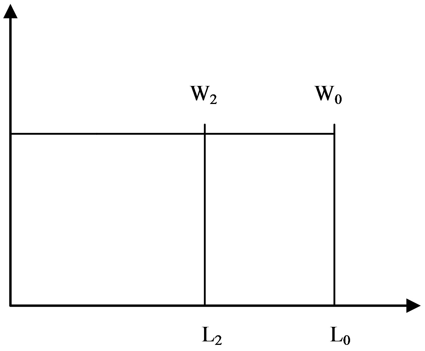
Figure 1. Keynes’s involuntary unemployment.

Figure 2. Walras’s voluntary unemployment.

Figure 3. Voluntary and involuntary unemployment.
unemployment and involuntary unemployment exist. The former is determined, as in the previous case, but the involuntary unemployment is the difference between L1 and L2. The total unemployment is the summation of these two kinds of unemployment, i.e., it is determined as (L0 – L1) + (L1 – L2) = (L0 – L2). Finally, let us consider two extreme forms of the supply curve: 1) If the supply curve is only a horizontal line (Figure 1), then there is either full employment if the equilibrium point is at the right boundary, or there is only involuntary unemployment, which is calculated as the difference between the boundary (available quantity) and equilibrium points (equilibrium employment). 2) If the supply curve is only a vertical line, there is full employment in all cases (Figure 4).
To sum up, Keynes’s original definition of types of unemployment, voluntary and involuntary, is very vague and unfinished; and did not allow calculating their magnitudes to use for employment policy. This is the fifth flaw of Keynes’s theory in the General Theory.
6. Keynes’s Multiplier
It is convenient that the multiplier is one of the central issues of Keynes’s GT. Blaug writes: ‘The principal novel prediction of Keynesian economics is that the value of the instantaneous multiplier is greater than unity’ [1, p. 189; 43, p. 40]. Moreover, two additional multipliers are also considered: the government-purchases multiplier and the tax multiplier. It has been claimed erroneously that on the one hand, an increase in government-purchases will raise the income, while on the other hand, an increase in tax will decrease the income, or alternatively, a decrease in tax will increase the income [44, pp. 253-257]. However at the same time, there were economists who indicated doubt regarding the multiplier [13, 46, and 49]. It is necessary to stress that Keynes stated that “The theory of the multiplier. … half the book is really about it” [28, p. 57].
The main argument of Keynes’s theory is that ‘when the genuine income of the community increases or decreases, its consumption will increase or decrease but not so fast’ [25, p. 114]. From this we can conclude that income is equivalent to the cause and consumption, as well as the saving (investment), is equivalent to effect.
Keynes continues ‘For ∆Yw = ∆Cw + ∆Iw, where ∆Cw and ∆Iw are the increments of consumption and investment; so that we can write ∆Yw = k∆Iw, where 1 – 1/k is equal to the marginal propensity to consume.
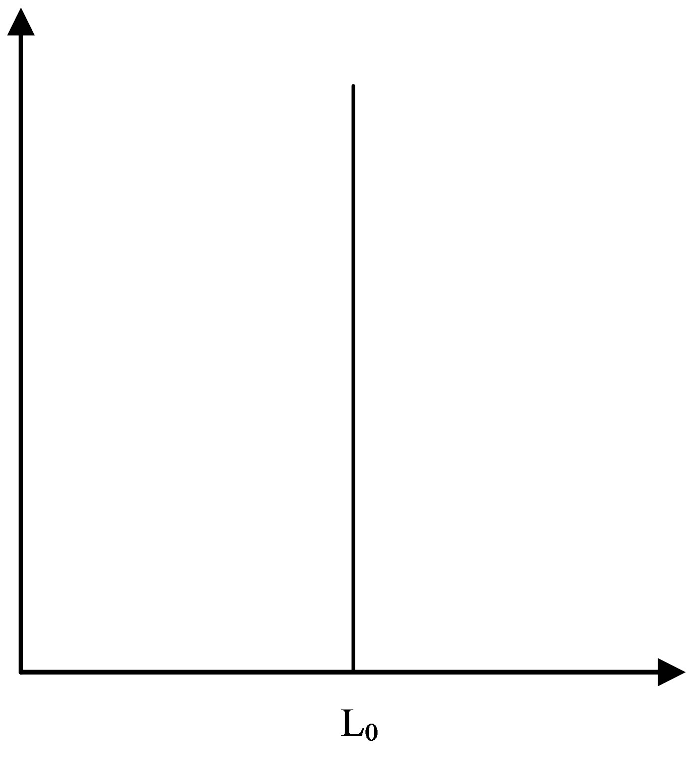
Figure 4. Full employment.
Let us call k the investment multiplier. It tells us that, when there is an increment of aggregate investment, income will increase by an amount which is k times the increment of investment [25, p. 115].
Here, Keynes made two incorrect suppositions. First, income and investment have been replaced; investment now becomes the cause and income the effect [13, p. 139, 45,46]. Moreover, investment is determinant, which is opposite Keynes’s statement “Saving and Investment are determinates’, in the first phase of the whole investment process which Keynes considered. However, the theory of causality teaches that such a replacement is generally incorrect and yields inadequate results [47,48].
Fortunately, such replacement may also be interpreted in a backward (reverse) direction. Namely, in order that the effect (investment) would occur, it is required (necessary and sufficient condition) that the cause (national income) would be occurred before. It is necessary to emphasize that this does not mean that the effect (investment) churns out the cause (national income); i.e., there is no replacement between the cause and the effect; it is simply the fact that in the case when the causal nexus is known, the backward causality allows us to determine the required cause in order that certain effect would be produced.
Second, Keynes’s “multiplier” is only a psychological phenomenon while the basic component-production, is omitted. Hence, we can conclude that k cannot be the multiplier.
On the other hand, Keynes’s “multiplier” is the inverse of the marginal propensity to invest [19,49,50]. This means that the rate of the multiplier depends on the marginal propensity to invest and the lower the latter, the higher the multiplier. For example, if the marginal propensity to invest is 0.1 then the rate of multiplier is 10, and if the first is 0.05, than the latter are 20. Consequently, to increase income is it better to consume than to save. So individuals were encouraged to spend on consumption and not save. Therefore, for the last twenty years the average propensity to invest in USA was decreased and reached 0.04 which means that the multiplier rate must be 25 [51]. Moreover, Hoover stated that “The expenditure multiplier is the intellectual basis for President Obama’s stimulus package” [52, p. 12].
On the other hand, the inverse of the marginal propensity to invest indicates the required quantities of income for a unit of investment, when the marginal propensity of both does not change. This result is compatible with the result of the backward (reverse) causality in the determination of the investment multiplier (vide supra). Therefore, the genuine meaning of Keynes’s multiplier is tantamount to a requirement, and not to a multiplication. Hence, the requirement indicates on the required quantity of national income for the realization of one unit of investment (saving) when the marginal propensity to consume is constant: “The multiplier tells us by how much their employment has to be increased to yield an increase in real income sufficient to induce them to do the necessary extra saving, and is a function of their psychological propensities” [25, p. 117; see also 9]. This means that an increase in consumption is not caused by the income that a new investment entails; except of an increase in investment and consumption which is produced by the income yields, by means of the available unemployed services (fixed capital and labor). Keynes’s following statement explicitly expresses this kind of interpretation to the multiplier: “According to the multiplier theory, there is an arithmetical relation between the level of consumption and the level of net investment, so that, other things being equal (i.e. nothing occurred to change the value of multiplier) consumption and net investment rise and fall in the same proportion” [28]. It is amazing that authors such as Keynes, Harrod, Hicks, and Samuelson termed it as a “multiplier”, which has to be source of multiplication, but actually meaning requirement!
According to such interpretation, using Keynes’s example again, in order to increase the investment by one, the income is required to increase by 10, where 9 units will be allocated to an increase in consumption. It must be stressed that the corresponding increase of income might not be possible at all, because of the limitations of unemployed services: labor, fixed capital, scarce raw materials, and so on [53].
Keynes’s followers have been trying to vindicate the “multiplier” and therefore, have been considered successsive-period (lagged or dynamic) multiplier according to Kahn, in parallel with his instantaneous (static) version [2,45]. However, there are two crucial differences between them. First, Keynes discussed closed economy where the source of the investment is the national income, while Kahn [54] considered open economy where the borrowing is the source of the investment increment. Second, in the latter case, to calculate net multiplier it is necessary to reduce the amount of repayment for borrowing from yielding increasing income.
Post-Keynes economists have extended the multiplier conception and introduced, firstly, government purchases (spending) multiplier, when modern authors even favorably dwell upon the option of taxes multiplier.
To sum up, Keynes’s multiplier’s genuine meaning is that of a requirement, which indicates the quantity of national income needed to realize one unit of investment. This is the sixth flaw of Keynes’s theory in the General Theory.
7. Money and Interest Rate in Keynes’s Theory
The money theory is an anchor of Keynes’s economic theory and his main contribution; and the source of Keynesian Revolution; “In other words, it was Keynes’s liquidity preference theory (LPT) of money that was the revolutionary aspect of Keynes’s analysis” [7, p. 172].
Keynes formulated the principal thesis of his theory as the following:
Thus the analysis of the Propensity to Consume, the definition of the Marginal Efficiency of Capital and the theory of the Rate of Interest are three main gaps in our existing knowledge, which it will be necessary to fill. When this has been accomplished, we shall find that the Theory of Prices falls into its proper place as a matter, which is subsidiary to our general theory. We discover, however, that Money plays an essential part in our theory of the Rate of Interest; and we shall attempt to disentangle the peculiar characteristics of Money, which distinguish it from other things [25, pp. 31-32].
So, Money and the Rate of Interest have to be crucial to Keynes’s theory and their correct interpretation and understanding is crucial for his whole theory [55].
Before discussing this, let us point out that Keynes, like Walras, used two types of money: money commodity (numéraire) and money. However, Keynes used the wage-unit as a numéraire, whilst Walras used precious metal (gold and silver). But using the wage-unit as a numéraire is very doubtful because of its determination: “the money-wage of a labour-unit we shall call the wageunit” [25, p. 41]). But, in our opinion, in fact Keynes as well as Marx used as a numéraire the labour-unit, which was used as a measure of the quantity of employment [ibid. p. 41; see also 5, p. 58]. In such a case there are two crucial problems. Firstly, whether labour might be used as a numéraire since in equilibrium state might be an unemployed part of labour? [56]. Secondly, labour is not homogeny and assuming that labour might be used as a numéraire then the question is what kind of labour is would be used? Keynes suggested using ‘an hour’s employment of ordinary labour as our unit and weighting an hour’s employment of special labour in proportion to its remuneration; an hour of special labour remunerated at double ordinary rates will count as two units’ [25, p. 41]. It is necessary to stress that, unfortunately, this is not as easy as Keynes described it. This is well known as an unsolved problem of the reduction of labour since Marx, who used the term “Abstract labour” and invested, in vain, huge energy to determine a unit of such labour. These problems are very acute when we consider a model including other services’ prices, such as the rent of land, the price of fixed capital’ service and the interest rate of money. As we have mentioned Keynes factually discussed the model with regards to one service—Labour and instead of that he discussed the problem of the marginal efficiency of capital and interest rate of money. This was in textual form and was not included in the model. Moreover, Marx used “abstract labour” only for the specific theoretical problem, namely for the problem connected to the Exploitation of the Workers’ Class. However, when Marx discussed problems of real economics he used only money measurement, while, Keynes used “wage-unit” for the real economic problem if we assume that Keynes’s economy is a real economy.
In addition, the use of labour (or wage-unit) as a numéraire is problematic, if impossible, because the numéraire is a basic component of the monetary system and it is used for all functions of money: exchange (transaction), measurement and storage. At the same time, it is necessary to note that Keynes used the term “gold standard” in the text of GT, but he never discussed the relationship between the wage-unit, the gold standard and paper money.
Nevertheless, in Keynes’s approach, as well as in Walras’s approach, aggregate demand of money is calculated on the basis of the individual’s decision [25, pp. 195, 198 and 199]. Unfortunately Keynes did not show how each individual reaches that decision, i.e., it is not clear how properties of individuals influence on the decision. Yet, it is not clear the connection with other economical categories (vide infra). Meanwhile, Keynes’s money theory is incomplete and even incorrect. Keynes continues:
Let the amount of cash held to satisfy the transactionsand precautionary-motives be M1, and the amount held to satisfy the speculative-motive be M2. Corresponding to these two compartments of cash, we then have two liquidity functions L1 and L2. L1 mainly depends on the level of income, whilst L2 mainly depends on the relation the current rate of the interest and the state of expectation. Thus M = M1 + M2 = L1(Y) + L2(r), [25, p. 199]
Here Keynes proposed two erroneous assumptions. First, Keynes merged the transaction-motive, which already represents a combination of the income-motive and the business-motive, with precautionary-motive. This eliminates the difference between two types of money: money as a medium of exchange, a measure of value and a store of value (the money commodity-numéraire) and money for circulation (the money commodity-numéraire, or fiat money), and therefore, consequently, the difference between two various prices for money commodity are also eliminated. This is the main reason that in modern economics only fiat money is used.
Second, Keynes asserted that L1—liquidity function of the amount of cash to satisfy the transactions-and precautionary-motives (M1) depends mainly on the level of income [M1 = L1(Y)]. Here, Keynes assumed that the liquidity function is the inverse function of the income function. Keynes used this approach very frequently, for example for the employment function, which is determined as the inverse function of the aggregate supply function [25, p. 280; Hicks also used this approach in his famous IS-LM model, see 57]. However, the inverse function exist only for the function of one variable with specific properties, namely, the function must be either strictly increasing or strictly decreasing function. Yet, the income function is the function for many variables (prices and available quantities for all categories—goods, factors of production (labour, fixed capital and money) and so on). Therefore, the assumption that the income function as the function of one variable, ones of money, ones of available quantities of either labour or fixed capital, is incorrect. What means that the liquidity function for the transactions-and precautionary-motives [M1 = L1(Y)] as the inverse function of the income function is not exist.
In the following Keynes surprisingly states that ‘In the static society in which for any other reason no one feels any uncertainty about the future rates of interest, the Liquidity Function L2, or the propensity to hoard (as we might term it), will always be zero in equilibrium. Hence in equilibrium M2 = 0 and M = M1;’ [25, p. 209]. But, this means that the rate of interest, crucial determinants, have disappeared in the equilibrium state! Keynes continues: “…so that any change in M will cause the rate of interest to fluctuate until income reaches a level at which the change in M1 is equal to the supposed change in M. Now M1 V = Y, where V is the income-velocity of money as defined above and Y is the aggregate income. Thus if it is practicable (our emphasis) to measure the quantity, O, and the price, P, of current output, we have Y = OP, and, therefore, MV = OP;” [ibid.].
There are some points to notice. Firstly, Keynes returns to the quantity theory of money. Secondly, we emphasized the word “practicable” because in chapter 4 Keynes states that “we cannot aggregate the Or’s, since åOr is not a numerical quantity [25, p. 45]”.
To sum up, Keynes’s money theory is incomplete and even incorrect. This is the seventh flaw of Keynes’s theory in the General Theory.
8. Conclusions
This paper revealed the seven flaws in Keynes’s General Theory which render it irrelevant and inapplicable to real world:
1) Keynes’s macro model is incomplete and imprecise; and the mathematical model for the individual economy is not formulated; and the adjustment (coordination) process between micro and macro economies is not discussed.
2) The amount of investment is generally determined by deducting the amount of consumption from the amount of income.
3) The aggregate functions of Keynes’s demand and supply, unfortunately, are incomplete; because they depend only on one variable, namely on the physical quantities of the given labour; in this case, the following variables are missing: wages; the fixed capital and its price; the land capital and its rent; circulation of capital and money for circulation and their prices.
4) The determination of the effective demand is unclear.
5) Keynes’s original definition of the types of unemployment, voluntary and involuntary, is very vague and unfinished; and does not allow us to calculate their magnitudes when we come to consider their implementation for an employment policy.
6) The genuine meaning of Keynes’s multiplier is that of a requirement, which indicates the quantity of the national income that is needed for the realization of one unit of investment.
7) Keynes’s money theory is incomplete and even incorrect.
REFERENCES
- M. Blaug, “Second Thoughts on the Keynesian Revolution,” In: B. J, Caldwell, The Philosophy and Methodology of Economics III, Edward Elgar, 1993.
- L. R. Klein, “The Keynesian Revolution,” Macmillan & Co LTD, London, 1952.
- P. A. Samuelson, “The General Theory,” In: R. Lekachman, Ed., Keynes’ General Theory Reports of Three Decades, ST Martin’s Press Macmillan & CO LTD, New York, 1964.
- R. Skidelski, “John Maynard Keynes,” Macmillan, London, 1996.
- V. Chick, “Macroeconomics after Keynes: A Reconsideration of the General Theory,” The MIT Press, Cambridge, 1983.
- R. W. Clower, “The Keynesian Counterrevolution: A Theoretical Appraisal,” In: F. H. Hahn and F. P. R. Brechling, Eds., The Theory of Interest Rate, Macmillan, London, 1965.
- P. Davidson, “Interpreting Keynes for the 21st Century,” Palgrave Macmillan, New York, 2007. http://dx.doi.org/10.1057/9780230286559
- G. C. Harcourt and P. A. Riach, “A ‘Second Edition’ of the General Theory,” Routledge, London, 1997.
- J. R. Hicks, “Mr. Keynes and the “Classics”: A Suggested Interpretation,” Econometrica, Vol. 5, No. 2, pp. 147-159.
- A. Leijonhufvud, “On Keynesian Economics and the Economics of Keynes,” Oxford University Press, New York, 1968.
- J. C. W. Ahiakpor, “Classical Macroeconomics Some Modern Variations and Distortions,” Routledge, London, 2003.
- F. A. Hayek, “Contra Keynes and Cambridge: Essays, Correspondence, Vol. IX, The Collected Works of F.”
- H. Hazlitt, “The Failure of the ‘New Economics’,” Van Nostrand, Princeton, 1937.
- B. W. Bateman, T. Hirai and M. C. Marcuzzo, “The Return to Keynes,” Harvard College, Harvard, 2010.
- P. Davidson, “The Keynes Solution,” Palgrave Macmillan, New York, 2009.
- P. Krugman, “How Did Economists Get It So Wrong?” The New York Times, 2009.
- J. Stiglitz, “The Triumphant Return of John Maynard Keynes,” Project Syndicate, 2008. http://www.project-syndicate.org/commentary/stiglitz107
- M. Hayes, “The Economics of Keynes: A New Guide to the General Theory,” 2010.
- D. Patinkin, “Money, Interest, and Prices,” 2nd Edition, MIT Press, Cambridge, 1989.
- P. Davidson, “A Keynesian View of Patinkin’s Theory, of Employment,” The Economic Journal, Vol. 77, No. 307, 1967, pp. 559-578.
- F. H. Hahn, “On Involuntary Unemployment,” The Economic Journal, Vol. 97, 1987, pp. 1-16.
- J. Robinson, “Economic Philosophy,” Anchor Books, New York, 1964.
- A. H. Meltzer, “On Keynes and Monetarism,” Worswik & Trewithick, 1983.
- T. Negishi, “History of Economic Theory,” North-Holland, New York, 1989.
- J. M. Keynes, “The General Theory of Employment Interest and Money,” Macmillan, London, 1936-1960.
- T. Negishi, “Microeconomic Foundations of Keynesian Macroeconomics,” North-Holland, New York, 1979.
- E. R. Weintraub, “Microfoundations: The Compatibility of Microeconomics and Macroeconomics,” Cambridge University Press, New York, 1979. http://dx.doi.org/10.1017/CBO9780511559570
- J. M. Keynes, “The Collective Writings of John Maynard Keynes,” In: D. Moggridge and S. T. Macmillan, Eds., The General Theory and After, Part II, Defense and Development, Martin’s Press, New York, 1973.
- M. Blaug, “Economic Theory in Retrospect,” 5th Edition, Cambridge University Press, Cambridge, 1996.
- L. Walras, “Elements of Pure Economics,” Allen and Unwin, London, 1954.
- E. J. Amadeo, “Keynes’s Principle of Effective Demand,” Edward Elgar Publisher, Aldershot, 1989.
- V. Chick, “The Nature of Keynesian Revolution: A Reassessment,” Australian Economic Papers, Vol. 17, No. 30, 1978, pp. 1-20. http://dx.doi.org/10.1111/j.1467-8454.1978.tb00607.x
- E. Davar, “Unemployment: Voluntary and Involuntary,” ASSA 2001 Conference, Atlanta, pp. 1-21.
- E. Davar, “The Genuine Meaning of Keynes’s Multiplier,” UK HET 2003 Conference, Leeds, 3-5 September 2003, pp. 1-25.
- M. De Vroey, “The History of Macroeconomics Viewed against the Background of the Marshall-Walras Divide,” The 2003 HOPE Conference, 2003, pp. 1-32.
- M. Morishima, “Walras’ Economics,” Cambridge University Press, Cambridge, 1977.
- R. Layard, S. Nickell and R. Jackman, “Unemployment, Macroeconomics Performance and the Labour Market,” Oxford University Press, Oxford, 1994.
- R. E. Lucas Jr., “Unemployment Policy,” The American Economic Review, Vol. 68, No. 2, 1978, pp. 353-357.
- C. A. Pissarides, “Equilibrium Unemployment Theory,” Basil Blackwell, Cambridge, 1990.
- J. B. Taylor, “Involuntary Unemployment,” In: J. Eatwell, M. Milgate and P. Newman, Eds., The New Palgrave Dictionary of Economics, Macmillan, Basingstoke, 1987, pp. 999-1001.
- C. Shapiro and J. E. Stiglitz, “Equilibrium Unemployment as a Worker-Discipline Device,” In: N. G. Mankiw and D. Romer, Eds., New Keynesian Economics, The MIT Press, Cambridge, 1991, pp. 123-141.
- J. D. Sachs and F. B. Larrain, “Macroeconomics in the Global Economy,” Prentice Hall, Englewood Cliffs, 1993.
- O. Lange, “Price Flexibility and Employment,” The Principia Press, Bloomington, 1944.
- N. G. Mankiw, “Macroeconomics,” 3rd Edition, Worth Publishers, New York, 1997.
- L. L. Pasinetti, “Growth and Income Distribution: Essays in Economic Theory,” Cambridge University Press, Cambridge, 1974.
- W. H. Stoddard, “The Algebra of John Maynard Keynes,” 2010. http://www.troynovant.com/Stoddard/Essays/Keynesian-Algebra.html
- E. Davar, “Flaws of Modern Economic Theory: The Origins of the Contemporary Financial-Economic Crisis,” Modern Economy, Vol. 2, No. 1, 2011, pp. 25-30. http://dx.doi.org/10.4236/me.2011.21004
- E. Davar, “Government Spending and Economic Growth,” The Finance and Business, No. 2, 2013, pp. 4-19.
- J. C. W. Ahiakpor, “Classical Macroeconomics: Some Modern Variations and Distortions,” Routledge, London, 2003.
- R. G. Hawtrey, “Capital and Employment,” Longmans, Green and Co., London, 1937.
- E. Davar, “Input-Output Analysis and Contemporary Economics,” Lambert Academic Publishing, Saarbrücken, 2013.
- K. D. Hoover, et al., “John Maynard Keynes of Bloomsbury: Four Short Talks,” Department of Economics, Duke University, Duke, 2009.
- J. R. Hicks, “The Crisis in Keynesian Economics,” Basil Blackwell, Oxford, 1974.
- R. Kahn, “The Relation of Home Investment to Unemployment,” Economic Journal, Vol. 41, No. 162, 1931, pp. 173-198. http://dx.doi.org/10.2307/2223697
- D. Laidler, “Fabricating the Keynesian Revolution,” Cambridge University Press, Cambridge, 1999.
- E. Davar, “The Renewal of Classical General Equilibrium Theory and Complete Input-Output System Models,” Avebury, Aldershot, Brookfield, Hong Kong, Singapore, Sydney, 1994.
- J. R. Hicks, “IS-LM: An Explanation,” Journal of Post Keynesian Economics, Vol. 3, No. 2, 1980-1981, pp. 139- 154.
- J. C. W. Ahiakpor, “Keynes and the Classics Reconsidered,” Kluwer, London, 1998.
- M. Boianovsky and H. M. Trautwein, “Wicksell, Cassel, and Idea of Involuntary Unemployment,” History of Political Economy, Vol. 35, No. 3, 2003, pp. 385-436.
- [61] R. G. Lipsey, P. O. Steiner, D. P. Douglas and P. N. Courant, “Economics,” 9th Edition, 1990.
- [62] W. A. Darity Jr. and B. L. Horn, “Involuntary Unemployment Reconsidered,” Southern Economic Journal, Vol. 49, No. 3, 1983, pp. 717-733. http://dx.doi.org/10.2307/1058712
- [63] J. Viner, “Mr. Keynes on the Causes of Unemployment 1936, Comment on My 1936 Review of Keynes General Theory,” In: R. Lekachman, Ed., Keynes’ General Theory, Reports of Three Decades, St Martin’s Press, Macmillan & Co Ltd, London, 1964.
- [64] B. Sheehan, “Understanding Keynes’s General Theory,” Palgrave Macmillan, New York, 2009. http://dx.doi.org/10.1057/9780230232853
- [65] A. Leijonhufvud, “Macroeconomic Instability and Coordination,” Edward Elgar, Northampton, 2000.
- [66] W. Young, “Interpreting Mr. Keynes,” Westview Press, Boulder, 1987.
- [67] D. Worswik and J. Trevithick, “Keynes and the Modern World,” Cambridge University Press, London, New York, 1983.
NOTES
1“It is doubtful, in fact, whether we would have got in such muddle over Keynes if we had understood Walras properly.” [32, note 32, p. 20].
2This is opposite to Hayes recent statement that ‘Keynes meant exactly what he wrote’ [18, p. xii].
3In the process of writing I encountered the place in the text of GT where Keynes used the term “effective supply” [25, pp. 231-232].
4It is interesting that Keynes in the final section of the Chapter 3 [25, pp. 32-34] discussed historical respective of effective demand and he did not mentioned Walras’ name.
5The notion “involuntary unemployment” was in use prior to Keynes both by English economists [54, pp. 19-20; 58] and also by other countries’ economists [59]. But their notion differs from Keynes’s notion.
6“For over half a century, economists have been trying to explain (or, in some cases, to deny the possibility of) involuntary unemployment. The subject is one of the most contentious and controversial in the discipline” [60, p. 751].
7“To us, involuntary unemployment is a real and important phenomenon with grave social consequences that needs to be explained and understood’ [17, p. 1217].
8“The approach taken in this book leads to the view that the decomposition of unemployment into frictional, cyclical, voluntary, involuntary, and so on is unhelpful in the theoretical and empirical analysis of unemployment” [39, xv-xvi].
9For example, Darity and Horn claim that “it is useful to demonstrate that Keynes’s unemployment equilibrium could be a Walrasian equilibrium” [61], p. 727].
10Viner claimed that “‘Voluntary’ unemployment is defined as the unemployment “due to refused or inability of a unit of labor... to accept a reward corresponding to the value of the product attributable to its marginal productivity,” but is used in such manner as to require the addition to this definition of the proviso…” [62, p. 236].
11For example, Sheehan’s recent determination of the involuntary unemployment: “The equilibrium volume of involuntary unemployment is equal to the difference between the full employment level and the actual level of employment” [63, p. 223; see also 18, p. 52].
12“This definition has been regarded as most tortuously contrived by most later interpreters” (Leijonhufvud, 1968, p. 94). “The term, without a doubt, is one of the most unfortunate new coinages in the history of economics” [64, 2000, p. 18].
13A quotation from Pigou’s letter (May 1937) to Keynes shows the priority Pigou gave to the correct definition of “involuntary unemployment” [28, p. 54].
Dear Keynes, I’ve looked up about Hawtrey p. 170, about which you asked me in the vac. My assumption was that, subject to the qualifications given on p. 7, the number of would-be wage earners is fixed independently of the stipulated wage. The supply schedule of labour is, therefore, like this: (see below) and, given perfect mobility, the quantity of unemployed is measured by the distance between the point where the demand curve cuts OP and P. If the stipulated wage is altered, the horizontal part of the curve moves to a lower or higher level, but the vertical part still passes through P.
14See Note 5 and [65,66].