Wireless Engineering and Technology
Vol.2 No.2(2011), Article ID:4731,6 pages DOI:10.4236/wet.2011.22016
A New Algorithm of Mobile Node Localization Based on RSSI
![]()
1College of Electrical and Information Engineering, Hunan University, Changsha, China; 2College of Information and Electrical Engineering, Hunan University of Science and Technology, Xiangtan, China.
Email: {JieZhanwl, kane.rex}@163.com, Hongliliu@vip.sina.com
Received March 8th, 2011; revised March 22nd, 2011; accepted March 25th, 2011.
Keywords: RSSI, wireless sensor networks, mobile location position, Signal Strength, weight
ABSTRACT
Position mobile node coordinate is a key component to determine the accuracy and efficiency of positioning in wireless sensor networks. Flexible location algorithm admits to adjust the accuracy and time cost of positioning based on the users references. This paper develops a location algorithm named Signal Strengthening Dynamic Value (SSDV) based on the database of RSSI to position the mobile node in terms of the value of beacon nodes RSSI. The proposed algorithm has successfully improved the accuracy of mobile nodes positioning and real-time, and simulation results show high performance in effectiveness of the algorithm.
1. Introduction
The algorithms of wireless sensor networks(WSN) position can be divided into two main categories [1]—Range-based position and Range-free position. in the Range-based position algorithm, we need to measure the distance and angle between the mobile nodes and the beacon nodes, and then count out the position of the mobile nodes by Tri-lateral measurements, Triangular measurements or Maximum likelihood estimation method. Yet, in the Range-free position algorithm, we need only information of the network-connectivity and signal strength. Here, non-distance-position method has a great superiority owing to that it has no requirements for accurate distance-measuring so that the cost of the hardware establishments will be greatly reduced and thus can be large-scale installed, and the precision of the position can be improved by algorithm. At present, the Range-free method has been widely used in the convex program [2], the DV-Hop [3] and etc. However, the convex program method requires that the reference nodes located on the edge of the network, otherwise the position will deflect towards the center; while the DV-Hop algorithm can carry out accurate position only in intensive isotropy networks [4]. The so-called isotropy here means that the signal strength will not change with the orientation of measures. However, it is hardly to guarantee the isotropy of the network in the indoor. Thus, the SSDV (Signal Strengthening Dynamic Value) scheme discussed in this article is born out of an algorithm of positioning which uses the Range-free techniques, and can accurately perceive the movements of the measuring objects. Thus it is very suitable to be used indoor. In our discussing, we assume that the wireless-signals can be kept steady and the signal covering scale of the nodes is a standard round area.
2. Principle of Distance Measurements of RSSI
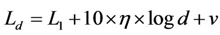
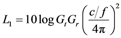
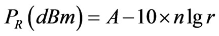
An important feather of wireless signal transmission is that the signal strength decreases as the distance increase. The principle of distance measurements of RSSI is to change attenuation of the signal strength into distance of signal transmission, using the functional relation between attenuation of the signal and the distance approximately. Researchers have done some effective researches about signals in different transmission environment [5], and conclude some good empirical formula:
 (1)
(1)
 (2)
(2)
 is Transmitting antenna gain,
  is Receiver antenna gain, c is velocity of light, f is carrier frequency,
  is Channel attenuation coefficient (2~6), v is the Gaussian random variable which considered the shadow effect, then v~
 , d is the distance,
  is the channel loss after the distance d.
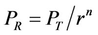
In practice, we get the relation between RSSI and the distance through the measurement of transmission power and receiving power. Most of the chips which provide RSSI measurement show the relation of transmission power and receiving power by the following formula: [6]
 (3)
(3)
After the conversion was:
 (4)
(4)
 is the receiving power of the wireless signal,
  is transmission power, n is the Propagation factor, r is the distance between Transceiver Unit. A is the receiving signal power when the signal transmit 1 meter. The numerical value of constant A and n determined the relation between receiving signal strength and signal transmission distance.
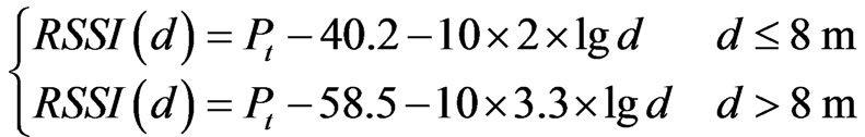
As to different chips, the empirical formula has corresponding different form due to different hardwire and modulation. The chip CC2430 used in our experiment is based on the IEEE802.15.4 agreement, using the DSSSO-QPSK modulation technology in the physical layer. IEEE802. 15. 4 gives the simplified channel model [7]
 (5)
(5)
Most of theoretical analysis and empirical formula show that the relationship between RSSI and the transmission distance of wireless signal is apparent. The measurement of RSSI has repeatability and interchange ability, and there is a pattern in the application environment when RSSI does appropriate changes. After having finished the environmental factors, RSSI can do the distance measurement of indoor and outdoor.
3. Ranging Experiment and Processing
In order to do a comprehensive discussion of RSSI ranging, we designed the following experiment. Do four groups ranging experiment which is mutually perpendicularity on an empty space, the nodes are above the ground one meter. The mobile node and fixed node start the ranging from the position one meter away, every 0.1 meter as a measuring point, and every measuring point will be measured 10 times. After 42 meters measured, part of the signals is not detected, because the RSSI values is obtained from complete receiving data packets, so the test is meaningless to continue. The four groups of experimental results are shown in the Figure 1.
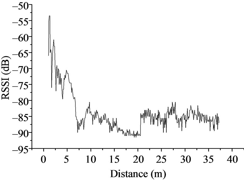
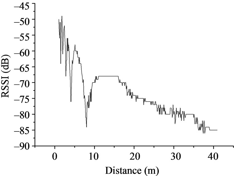
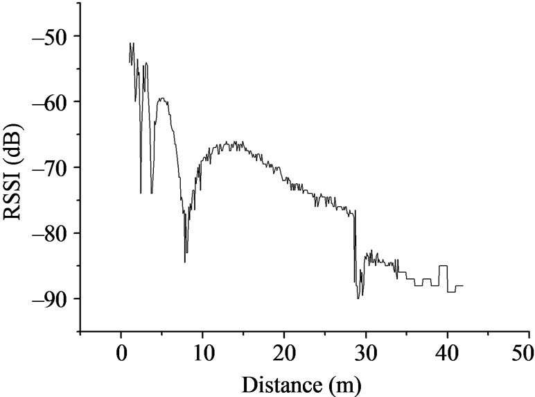
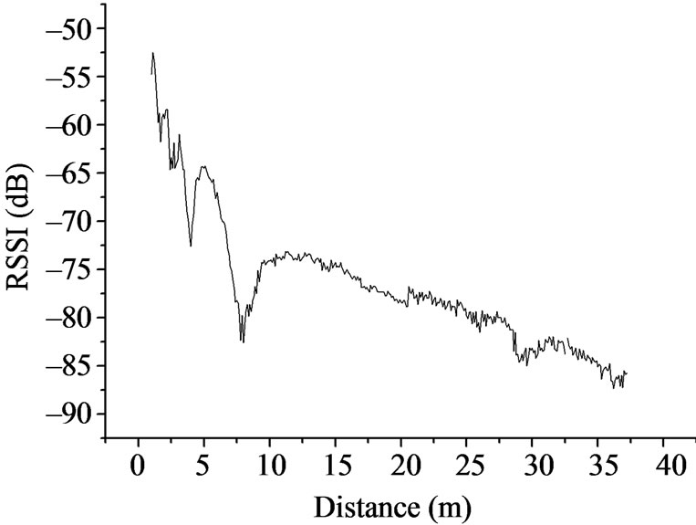
Figure 1. The measured value of RSSI vs. distance.
We have collected 16000 experimental data, and the analysis on those statistics shows that: Each RSSI value corresponds to an distance scope, and high-intensity values has small probability, low-intensity values has large probability. So we can find the highest density peaks and filter out most wrong dates by doing Gaussian fitting. The probability distribution Restructure is shown in the Figure 2. There is only one peak for each different RSSI measurement value, and the peak is steeper as the value is bigger, then the error is small, the peak is more slowly as the value is smaller, then the error become big. We get the fitting function:
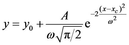 (6)
(6)
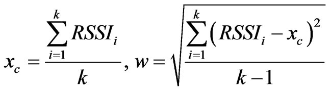
It is hard to find out the RSSI peak value of each measurement point. The value can be substituted into (6), when 0.5 ≤ y ≤ 1,we consider it is a large probability event and can be reserved, then we obtain the determined RSSI value by taking the average of the reserved RSSI values.  and A are undetermined coefficients(can be determined by the relation between beacon nodes’ location and RSSI), k is the number of received beacon nodes.
Gaussian fitting reduced the influence of some low probability and large disturbance events by using Gaussian fitting to do data processing, and reduced the ranging error. Figure 3 is the data processing results compared to Gaussian fitting and mean approach. The result shows that Gaussian fitting is better than mean model in improving ranging precise, especially when we measure close distance, and the error can be control within 1.2 meters on open space.
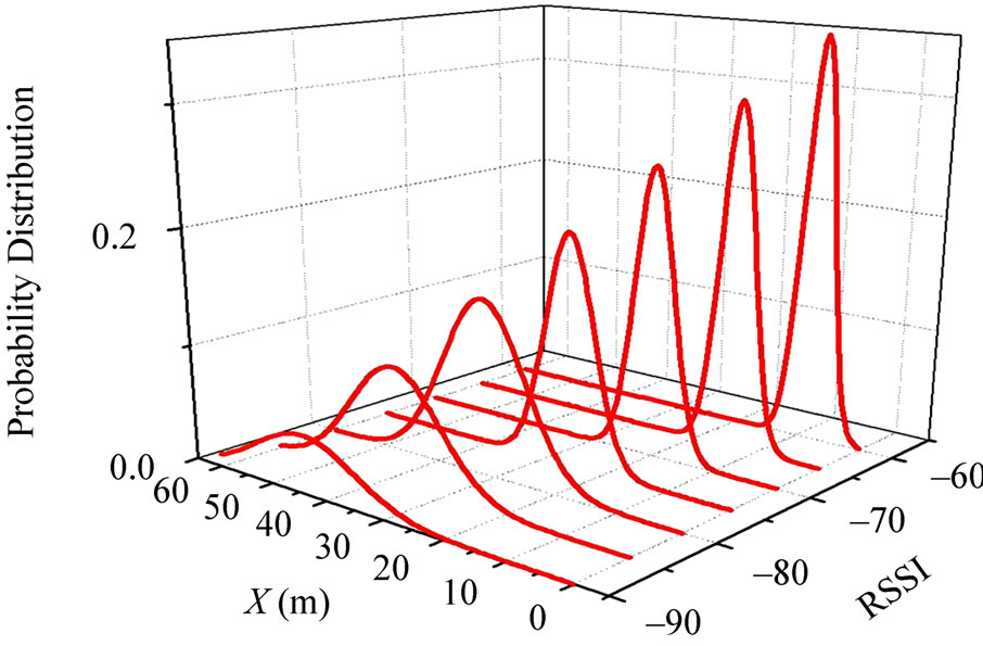
Figure 2. Probability distribution of RSSI by Gaussian fitting.
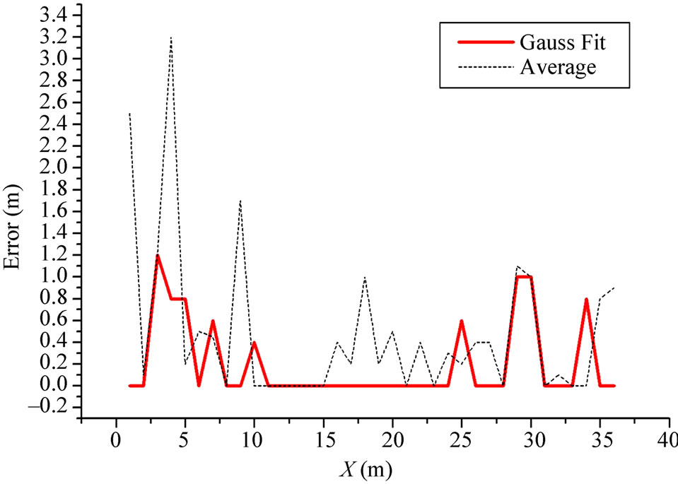
Figure 3. The distribution error of Gaussian fitting vs. average.
4. The Signal Strengthen Dynamic Value Scheme (SSDV)
4.1. The Principle of Position
First, the SSDV builds up the data-base of the reference nodes via the exchange nodes which keep on sending out signals, signals are received by the reference nodes and then the reference nodes send back information of the strength of the signals. Shown as figure 4, the exchange nodes keep broadcasting signals which carry information of its ID and all the reference nodes and exchange nodes receive the signals and send back information of the signals which it received and information of its own ID. With the data-base of the reference nodes, the positioning scheme can work even without reference nodes. When a mobile node needs to be positioned, it will send information of the signal strength of all the exchange nodes that it can receive together with a position requirement. The position procedure is as follows:
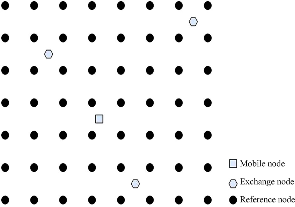
Figure 4. The structure and principle of positioning system.
Suppose the mobile node as X, and 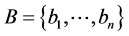 as all the exchange nodes that can be detected by X, the strength of the signals that X receives as
 ,
,  as all the reference nodes in the positioning region. As to every random
 , the signal strength of the exchange nodes received are supposed as
 , du, dv are the two adjacent reference nodes;
 ,
,  ,
,  is supposed as the focus reference nodes; let
 ,
,  is supposed as the assistant positioning-line that connects du and dv, and the value is expressed as
 ; and
; and  is the minimum rectangle region which is formed by 4 reference nodes in the positioning region. Here, we consider them as clusters. Let
 ,
,  ,
,  , then
  stands for the focus clusters; let
 , then
 .
.
Step 1: Find out the two key exchange nodes. Suppose that ,
,  when
when , then the
  is the kernel exchange node for the mobile nodes; if the
 ,
,  when
when , the
, the  is the terminus exchange node;
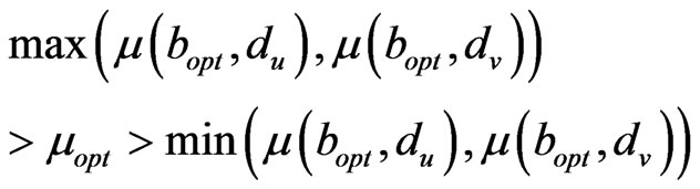
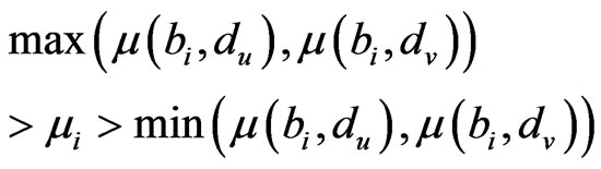
Step 2: Find out all the focus nodes in the positioning region. When  can assure that
 (7)
(7)
consider the assistant positioning-line that connects the couple of ,
,  as
as , then all the
  are focus clusters and when we judge all the
 ,
,  in the positioning region using Formula (2), we will get the HD and HC of the positioning region;
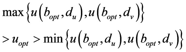
Step 3: Test whether X is positioned in the region. As for every randomly couple ,
,  , let
, let ,
,  , the following formula is:
 (8)
(8)
then it means that X is positioned in the region and the positioning can go on; if there are no couples of ,
,  ,
,  ,
,  accord with the Formula (8), it means that X is not positioned in the region and thus end the positioning procedure.
Step 4: Carry on the matching step. If there exists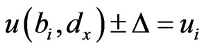 ,
,  , where the
  is a threshold value which is used to balance the errors brought by interference, then the position of
  is the position of the mobile node and the position is ended. Otherwise, the position goes on.
Step 5: Calculate the value of the focus clusters. As for all ,
,  ,
,  ,
,  , and
, and , let the following formula:
 (9)
(9)
come into existence for k times, then the value of the assistant positioning-line which connects the couple of ,
,  expressed as
  is k. All the values of
  to be calculated by Formula (9). Then, all
  can be calculated by formula:
 .
.
Step 6: Carry on the matching step of clusters. If there exists an exclusive ,
,  , then the center of this maximum cluster is the position of the mobile node and the position ends up; if
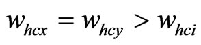 ,
,  , at meantime,
  and
and  are adjacent clusters, then the center of the cluster made up by these two clusters is the position of the mobile node and the position ends up.
4.2. The Characteristic of the Algorithm
Figure 5 is the sketch map of the position. In circumstances as shown in the figure, A, B, C stand for exchange nodes and C is the nuclear exchange node, A is the terminus exchange node; let M1, M2 be mobile nodes to be positioned, the small dots stand for reference nodes among which the brightened ones stand for hot clusters.
1) No blind spot in the positioning region. After the node-matching and the cluster-matching steps, the blind spots can be completely cleared up and this makes the originally unhandy Mass-Center Position Scheme much more flexible in that the positioning spot is not limited to only the mass center of the cluster but also the midpoint of the assistant positioning-line and places of reference nodes. Thus, the accuracy of the positioning will increased greatly.
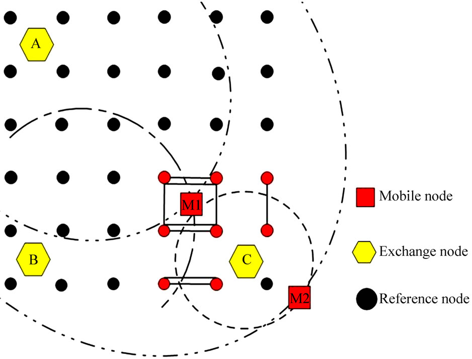
Figure 5. The sketch map of the positioning of SSDV.
2) Good real-time effect of positioning. Via the determining of hot cluster, the quantity of unnecessary calculations will be greatly cut. As shown in Figure 1, when positioning M1, it needs only to calculate the value of the cluster in the right-foot of the whole positioning region but no needs for any other ones.
3) Be able to determine whether the mobile node is positioned in the region. Via comparing the value of the assistant positioning–line produced by the terminus exchange nodes with the value of the assistant positioning-line produced by the nuclear exchange node, it is able to determine whether the mobile node is positioned in the positioning region. As shown in Figure 3, when positioning M2, although the nuclear exchange node C can still produce a hot cluster in region shown in the figure, however, as the terminus exchange node A does not bring out any value in the focus cluster, we can still determine that M2 is not positioned in the region.
5. Simulation Analysis
Suppose the positioning region is a square plane with an area of 50 × 50 m2, and on it an square region with an area of 40 × 40 m2 is distributed equably with reference region and the space between the reference nodes is 5 m. the exchange nodes are positioned in the four point angles A, B, C, D of the positioning region.
The simulation result is shown in figure 6. The black line is the assistant positioning-line, the larger the value, the wider the line. The assistant with no value will not be shown. And the triangular shapes refer the focus reference nodes region while the small square shapes refer the actual spot of the mobile nodes, and the stars are the places that are determined by calculation. In figure 6(a), the mobile node is positioned at coordinate (41, 39). The positioning result which is calculated by node-matching is coordinate (40, 40) with an error of 1.4142 m and timecost of 28 ms. In figure 6(b), the mobile node is positioned at coordinate (26, 28), and the calculated positioning result is coordinate (25, 27.5) with an error of 1.118 m and time-cost of 43 ms. In figure 6(c), the mobile node is positioned at coordinate (13, 17), and the calculated positioning result is coordinate(12.5, 17.5) with an error of 0.7071 m and time-cost of 41 ms. In figure 6(d), the mobile node is positioned at coordinate (48, 24), and the calculated positioning result shows that it does not exist in the positioning region with a time-cost of 29 ms.
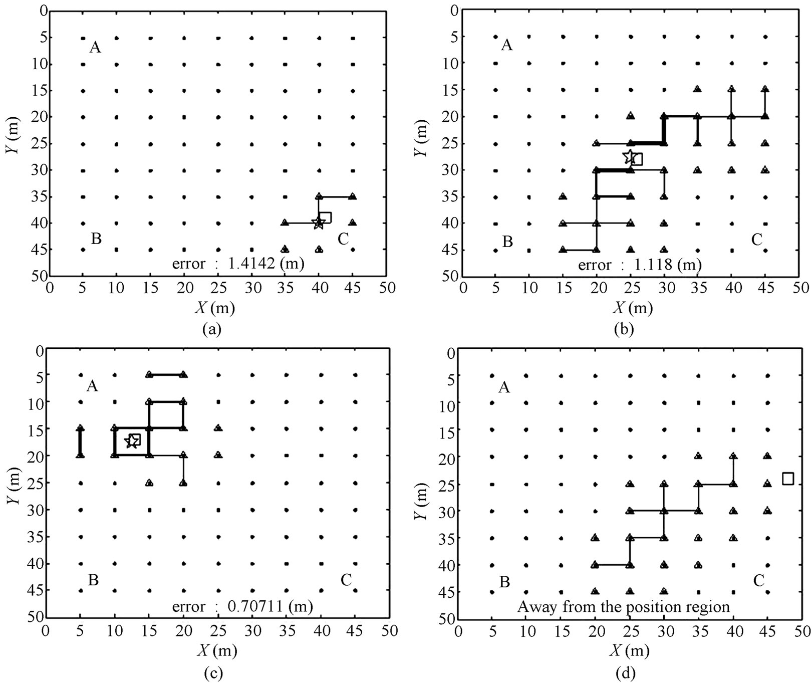
Figure 6. Simulated positioning result of SSDV.
From figures 6(a) and (b), we can see that the SSDV can determine the mobile nodes on special positions accurately; As from figure 6(c), it shows that most mobile nodes on normal positions can be determined accurately by this algorithm. From figure 6(d), we can see that when the mobile node is located out of the positioning region, the SSDV can find this out correctly. While comparing (a), (d) with (b), (c), we can see that the less the steps of the positioning, the less of the time-cost; while comparing (b) with (c), we can see that the closer is the mobile node near to any random reference node, the smaller the focus positioning region will be while the time cost is cut only with a very small quantity. On the contrary, the focus positioning region will get larger and the time-cost increase also has a very little quantity.
6. Conclusions
This paper presents a new algorithm of SSDV. This algorithm needs only the strength of the radio signals as foundation to position the mobile nodes. The establishment is rather simple and there is no blind spot in positioning region, and the accuracy and the time of positioning can both be adjusted by the users. The result of simulation proves the validity of this algorithm.
REFERENCES
- F. B. Wang, L. Shi and F. Y. Ren, “Self-Localization Systems and Algorithms for Wireless Sensor Networks,” Journal of Software, Vol. 16, No. 5, 2005, pp. 857-868. doi:10.1360/jos160857
- L Doherty, K. S. J. Pister and L. E. Ghaoui, “Convex Position Estimation in Wireless Sensor Networks,” Proceedings of the 20th Annual Joint Conference of the IEEE Computer and Communications Societies, Anchorage, Vol. 3, 22-26 April 2001, pp. 1655-1663. doi:10.1023/A:1023403323460
- D. Niculescu and B. Nath, “DV Based Positioning in Ad Hoc Networks,” Journal of Telecommunication Systems, Vol. 22, No. 4, 2003, pp. 267-280.
- M.-H. Jin, E. H.-K. Wu, Y.-B. Liao and H.-C. Liao, “802.11-Based Positioning System for Context Aware Applications,” Proceedings of Global Telecommunications Conference, Vol. 2, 1-5 December 2003, pp. 929- 933.
- L. Girod and D. Estrin, “Robust Range Estimation Using Acoustic and Multimodal Sensing,” Proceedings of the IEEE/RSJ International Conference on Intelligent Robots and Systems, Maui, 29 October-3 November 2001, pp. 1312-1320.
- L. Girod, V. Bychovskiy, J. Elson and D. Estrin, “Locating Tiny Sensors in Time and Space: A Case Study,” In: B. Werner, Ed., Proceedings of the IEEE International Conference on Computer Design: VLSI in Computers and Processors, Freiburg, 16-18 September 2002, pp. 214-219.
- J. Zhan, L.-X. Wu and Z.-J. Tang, “Research on Ranging Accuracy Based on RSSI of Wireless Sensor Network,” Telecommunication Engineering, Vol. 50, No. 4, 2010, pp. 83-87.
NOTES
Foundation Item: Hunan Provincial Science and Technology Plan Project (No.2010FJ4068); National Laboratory for Infrared Physics, Chinese Academy of Sciences (201021).