Journal of Environmental Protection
Vol. 3 No. 6 (2012) , Article ID: 20077 , 14 pages DOI:10.4236/jep.2012.36065
Trend Analysis of the Mean Annual Temperature in Rwanda during the Last Fifty Two Years
![]()
Department of Physics, National University of Rwanda, Butare, Rwanda.
Email: bsafari@nur.ac.rw
Received March 21st, 2012; revised April 13th, 2012; accepted May 16th, 2012
Keywords: Climate Change; Global Warming; Trend Detection; Mann-Kendall Rank Statistic Test; CUSUM and Bootstrapping; Temperature; Rwanda
ABSTRACT
Climate change and global warming are widely recognized as the most significant environmental dilemma the world is experiencing today. Recent studies have shown that the Earth’s surface air temperature has increased by 0.6˚C - 0.8˚C during the 20th century, along with changes in the hydrological cycle. This has alerted the international community and brought great interest to climate scientists leading to several studies on climate trend detection at various scales. This paper examines the long-term modification of the near surface air temperature in Rwanda. Time series of near surface air temperature data for the period ranging from 1958 to 2010 for five weather observatories were collected from the Rwanda National Meteorological Service. Variations and trends of annual mean temperature time series were examined. The cumulative sum charts (CUSUM) and bootstrapping and the sequential version of the Mann Kendall Rank Statistic were used for the detection of abrupt changes. Regression analysis was performed for the trends and the Mann-Kendall Rank Statistic Test was used for the examination of their significance. Statistically significant abrupt changes and trends have been detected. The major change point in the annual mean temperature occurred around 1977-1979. The analysis of the annual mean temperature showed for all observatories a not very significant cooling trend during the period ranging from 1958 to 1977-1979 while a significant warming trend was furthermore observed for the period after the 1977- 1979 where Kigali, the Capital of Rwanda, presented the highest values of the slope (0.0455/year) with high value of coefficient of determination (R2 = 0.6798), the Kendall’s tau statistic (M-K = 0.62), the Kendall Score (S = 328) with a two-sided p-value far less than the confidence level α of 5%. This is most likely explained by the growing population and increasing urbanization and industrialization the country has experienced, especially the Capital City Kigali, during the last decades.
1. Introduction
Climate change and global warming are worldwide recognized as the most significant environmental dilemma the world is experiencing today [1-4]. Concern in climate change and global warming by the international community, non-government organizations and governments has brought great interest to climate scientists leading to several studies on climate trend detection at global, hemispherical and regional scales [5-7]. Climate change and global warming are commonly detected throughout studies of variability of climatic parameters such as rainfall, temperature, lake’s level, runoff and groundwater. Nowadays, study of long-term temperature variability has been a topic of particular attention for climate researchers as temperature affects straightaway human activities in all domains. Increase in anthropogenic greenhouse gases’ concentrations in the atmosphere mainly due to human activities such as deforestation and burning fossil fuel and the conversion of the Earth’s land to urban uses driven largely by the rapid growth of the Earth’s human population are one of the causes of the warming of the climate system and of the process of climate change in several regions of the planet [8].
Several studies of long-term time series of temperatures have been done on a hemispherical and global scale [9-12]. Results have shown that the Earth’s surface air temperature has increased by 0.6˚C - 0.8˚C during the 20th century, along with changes in the hydrologic cycle. Temperatures in the lower troposphere have increased between 0.13˚C and 0.22˚C per decade since 1979, according to satellite temperature measurements [13]. In an analysis of a time series combining global land and marine surface temperature record from 1850 to 2010 developed by the Climate Research Unit (CRU), the year 2005 was seen as the second warmest year, behind 1998 with 2003 and 2010 tied for third warmest year [9,14].
Some other studies have been done on regional scale and have indicated that significant trends in observed temperatures have occurred during the second half of the 20th century and that the increasing has persisted, among others in Europe [15-18], in North America [19-21], in Arab countries [22-25], in Africa [26-34].
In a recent study on the African Continent [35], using Microwave Sounding Unit (MSU) total lower-tropospheric temperature data from the Remote Sensing Systems (RSS) and the University of Alabama in Huntsville (UAH) datasets, significant increasing temperature trends were found on the average in all of Africa Continent, Northern Hemisphere Africa, Southern Hemisphere Africa, tropical Africa, and subtropical Africa. The two most recent decades were compared with the period 1979-1990. Warming was observed over these same regions and was concentrated in the most recent decade, from 2001 to 2010. The results were likely attributed to other natural variability of the climate and/or to human activity but not to the El Niño-Southern Oscillation as previously suggested by other authors [31,36]. Generally, there is consent by scientists that most of the observed increase in globally averaged temperatures since the mid-20th century is unequivocal and very likely due to the observed increase in anthropogenic greenhouse gas concentrations. The 10 warmest years of the 20th century all occurred in the last 15 years of the century, 1998 being the warmest year on record. The Intergovernmental Panel on Climate Change (IPCC) projected that the average global surface temperatures will continue to increase to between 1.4˚C to 5.8˚C above 1990 levels, by 2100 [2]. To some extent, other factors such as variations in solar radiation [11] and at regional scale, land use are also considered to be among the causes of the observed global warming [28,37-43].
Though some studies have been done on climate change in different regions of Africa and the whole continent, the lack of reliable surface observational climate data still constitute a foremost gap affecting the detection capacity of impacts resulting from long-term climate changes. An effort is therefore required in maintaining existing observatories and increasing networks, and cooperation between countries. Regardless of the limited surface observational climate data, results from those studies indicate in general an increasing trend in temperature and a decreasing trend in rainfall during the last century. The implications of the observed climatic changes on the economy of the African developing countries, Rwanda in particular, are gigantic. In consequence, the effects of those changes necessitate to be taken into consideration and to be integrated in future planning programmes. In Rwanda, few scientific studies have been done on climatic change despite the good determination of the Government. This is mainly due to scarcity of research capacity in that domain, one of consequences of Rwanda history.
2. Study Area
Rwanda is a small mountainous, landlocked country in the Great Lakes region of Africa. Bordered by the Democratic Republic of the Congo (DRC), Burundi, Tanzania and Uganda, it is located at 02˚00 Latitude South and 30˚00 Longitude East. Total land area is about 24,950 km2, and inland lakes cover about 1390 km2. Because of the high altitude of the country, Rwanda has a pleasing moderate and tropical climate. Temperature in Rwanda varies throughout the year with two maxima and two minima. The low maximum temperature occurs in February while the high maximum temperature occurs in August. The two minima occur respectively in June and in November. The average temperature for Rwanda is around 20˚C and varies with the topography. The warmest annual average temperatures are found in the eastern plateau (20˚C - 21˚C) and south-eastern valley of Rusizi (23˚C - 24˚C), and cooler temperatures are found in higher elevations of the central plateau (17.5˚C - 19˚C) and highlands (<17˚C). Annual rainfall varies across the country, with the highest totals in the western part and the high elevated north-western part (>1200 mm) and then diminishing towards the eastern plateau (<900 mm). The country experiences two rainy seasons in a year associated with the North-South oscillating migration of the InterTropical Convergence Zone (ITCZ) of trade winds. The period of March, April and May corresponds to the long rainy season when the ITCZ moves to the North and the period of October, November and December to the short rainy season when the ITCZ returns to the South. A short dry season occurs from January to February and a long dry season from June to September.
Rwanda’s population is 11,370,425 and its population density, 416 people per square kilometer, is amongst the highest in Africa with a growth rate of 2.8% per year. Currently, 14% of the Rwandan population have access to electricity, though this is concentrated in the Capital City, Kigali. In rural areas where the majority of population lives, there remains limited access to electric power. Rwanda’s land area covered by forest is 20% and biomass (wood, agriculture residues, charcoal, peat and organic gas) is the major source of energy compared to fuel and electricity. Wood and charcoal energy are used by more than 90% of the population. During the last two decades, Rwanda has known an increasing urbanization at a rate of 4.4% per year. The increasing population and the intensified urbanization combined with the effect of climate changes have influenced Rwanda’s socio-economic by causing pressure on land, water, food and energy resources.
Recently, Rwanda has experienced heavy floods caused by severe torrential rain that have damaged villages located in the mountainous northern part of the country killing people and destroying hundreds of homes. Rainfall patterns, and beginning and end of rainfall season have been erratic with the consequence that cultivators were confused as to when to plant and harvest. There are some indications that Rwanda has been subject to climate change. Observations from the National Meteorological Service have indicated that during the last 30 years minimum temperature has risen up to two degrees. The year 2005 was the hottest year for many years in Rwanda. Minimum temperature climbed to 20.4˚C in August and maximum temperature climbed to 35˚C in the Capital City, Kigali.
The objective of the present study was to examine the long-term modification of the near surface air temperature in Rwanda.
3. Data and Method
3.1. Data
The data used in this study were collected from the Rwanda National Meteorological Service. They consisted of time series of daily data of near surface mean air temperature for the period ranging from 1958 to 2010 for five weather observatories as shown in Figure 1, Figure 2 and Table 1.
Those data were statistically processed and then reduced to annual mean values for further analysis.
Data Processing and Adjustment
Studies of long-term climate change require that data be homogenous. Observed climate abrupt changes in a homogenous climate time series are caused only by variations in weather and climate [44].
The major sources of errors in the detection of abrupt changes in climate data often consist of change of location of observatory, changes of instruments, change in observation times, missing data, methods used to calculate daily means and increased urbanized and or industrialized areas. Inhomogeneities in climate data time series can bring inaccuracies and make possible misinterpretation in the investigation of climate change over a region when analyzing a given climate parameter. Several studies have been conducted on quality control and homogenization of climatological data for the detection of climate
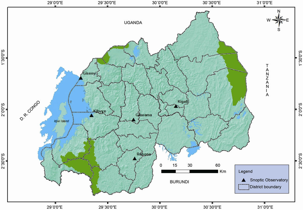
Figure 1. Geographical locations of the five synoptic observatories.
trends, and detailed explanations on the procedures to be followed for adjusting missing data were given [45-53]. In the present study, the Short-cut Bartlett homogeneity test was applied to the mean annual temperature data for the period of 1971-1980, considered as a reference period, where observations were concurrently measured at all observatories. The test showed that the data were homogeneous for the five observatories. The values of Pearson correlation coefficients (P.C.C.) were computed for the observed mean annual temperatures at the five observatories for the reference period in order to identify the best correlated observatories. Table 2 presents observatories which were found to be highly correlated with a p-value lower than the significance level . Missing values for the long period 1958-2010 were then adjusted by values computed from interpolation.
Missing data in the time series for an observatory Ofor a period ranging from year  to year
 , were completed by interpolated values
  obtained from observed data
  from another highly correlated observatory O using the equation of regression derived from the reference period of observation. Regressions of adjusted long-term time series of mean annual temperature data for the five observatories are presented in Figure 3. Long term time series of mean annual temperature were generated as presented in Figure 4.
3.2. Method for Abrupt Changes and Trends Detection
Variations and trends of annual mean temperature values time series were examined. The cumulative sum charts (CUSUM) and bootstrapping and the sequential version of the Mann Kendall Rank Statistic were used for the
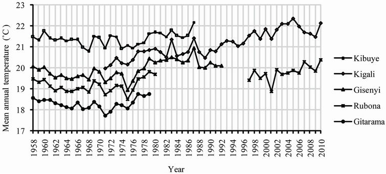
Figure 2. Time series of observed mean annual temperature (˚C).
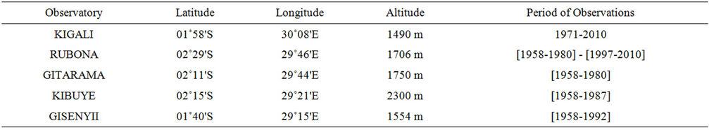
Table 1. Geographic coordinates of the five weather observatories and periods of observations.
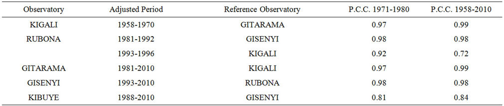
Table 2. Adjusted period and Pearson correlation coefficients (P.C.C.) for observed mean annual temperatures at the five observatories for the reference period 1971-1980 and for the whole period of study 1958-2010 after adjustments.
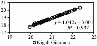
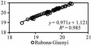
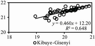
Figure 3. Regressions of adjusted long-term time series of mean annual temperature data (1958-2010) for the five observatories.
detection of abrupt changes. Regression analysis was performed for the trends and the Mann-Kendall Rank Statistic Test was used for the examination of their significance.
3.2.1. Cumulative Sum Charts (CUSUM) and Bootstrapping
The cumulative sum charts (CUSUM) and bootstrapping procedure was performed as suggested by Taylor [54]. Let  represent N data points of a time series,
  are iteratively computed as follows:
1) The average  of
of  is given by
 (1)
(1)
2) Let  be equal to zero 3) Compute
  recursively as follows:

 (2)
(2)
A section of the CUSUM chart with an increasing slope will indicate a period of time where the values tend to be above the overall average. Likewise, a section with a decreasing slope will indicate a period of time where the values tend to be below the overall average. The confidence level can be determined by performing bootstrap analysis [55-57].
3.2.2. Mann Kendal Rank Statistic
There are a number of statistical tests that are used for the analysis of trend such as Spearman rank statistic test, Cramer’s test, Pearson’s test, Pettit’s test, Buishand’s test, Von Neumann’s test, Standard normal homogeneity test (SNHT), Mann Kendall’s Rank Statistic test. The latest is considered to be the most appropriate for the analysis of climatic changes in climatological time series or for the detection of climatic abrupt changes [58].
The data were analyzed in order to identify significant long-term trends using sequential version of the MannKendall rank statistics, the effective application of which includes the following steps in sequence:
i) The values  of the original series are replaced by their ranks
  arranged in ascending order
ii) The magnitudes of , (
, ( ) are compared with
 , (
, ( ). At each comparison number of cases
  is counted and denoted by
 .
.
iii) A statistic  is, therefore, defined as follows:
 (3)
(3)
iv) The distribution of the test statistic  has a mean and a variance as
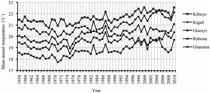
Figure 4. Time series of adjusted mean annual temperature (˚C) for the period 1958-2010.
and
 (5)
(5)
v) The sequential values of the statistic  are then computed as
 (6)
(6)
Herein,  is a standardized variable that has zero mean and unit standard deviation, and there-fore, its sequential behavior fluctuates around zero level. Furthermore,
  follows a Gaussian normal distribution.
vi) Similarly, the values of  are computed backward starting from the end of the series.
The intersection of the curves  and
and  localizes the change (in fact this change represents an abrupt climatic change) and allows the identification of the year when a trend or change initiates. When the values of
  are higher—in absolute value—than 1.96, it implies a trend or a change in the time series. In the absence of any trend in the series, the graphical representation of
  and
and  gives curves which overlap several times.
3.2.3. Kendall Rank Correlation
Let  be a set of joint observations from two random variables X and Y respectively, such that all the values of the couple (xi, yi) are unique. Any pair of observations (xi, yi) and (xj, yj) are said to be concordant if the ranks for both elements agree: that is, if both xi > xj and yi > yj or if both xi < xj and yi < yj. They are said to be discordant, if xi > xj and yi < yj or if xi < xj and yi > yj. If xi = xj or yi = yj, the pair is neither concordant, nor discordant. Kendall’s rank correlation measures the strength of monotonic association between the vectors X and Y.
In the case of no ties in the X and Y variables, if N represents the number of concordant pairs and M represents the number of discordant pairs, Kendall’s rank correlation coefficient τ is defined as:
 (7)
(7)
or
 (8)
(8)
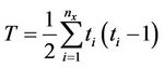
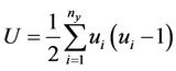
where S, is the Kendall score given by:
 (9)
(9)
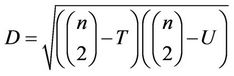
where  denotes the sign function and D is the maximum possible value of S. In the case where there are no ties among either the (xi) or the (yi),
 (10)
(10)
D is called the denominator and corresponds to the total number of pairs, so the coefficient  must be in the range [–1, +1]. If the agreement between the two rankings is perfect (i.e., the two rankings are the same) the coefficient has value 1. If the disagreement between the two rankings is perfect (i.e., one ranking is the reverse of the other) the coefficient has value –1. If X and Y are independent, then we would expect the coefficient to be approximately zero.
More general, if there are  distinct ties of extent
 ,
,  among the (xi) and
  distinct ties of extent
 ,
,  among the (yi) then:
 (11)
(11)
where
 (12)
(12)
and
 (13)
(13)
In the case where there are no ties in either ranking, it is well known that under the null hypothesis that there is no trend in the data i.e. no correlation between considered variable X and Y, each ordering of the dataset is equally likely, the statistic S may be well approximated by a normal distribution with the mean  and the variance
  as follows:
 (14)
(14)
 (15)
(15)
provided that .
.
For situation where ties occur, then  is extended to a more complicated including form adjusting terms for tied or censored data:
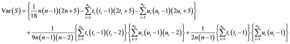 (16)
(16)
For trend test, the variable Y can be time. The presence of statistically significant trend is evaluated using the Z value. This statistic is used to test the null hypothesis such that no trend exists. The standardized test statistic Z is given by:
 (17)
(17)
A positive Z indicates an increasing trend in the timeseries, while a negative Z indicates a decreasing trend. To test for either increasing or decreasing monotonic trend at P significant level, the null hypothesis  is rejected if the absolute value of Z is greater than
 , where
  is obtained from the standard normal cumulative distribution tables and represents the standard normal deviates and p is the significant level for the test. The test of the null hypothesis H0:τ = 0 is equivalent to testing H0:Z = 0.
3.2.4. Regression Analysis
A simple linear regression model was applied to show the long-term annual trends in temperature for the periods of study. Change in temperature over the study period given by the estimated slope of the regression line and the coefficient of determination ( ) were computed from the regression model [59]. The Mann-Kendall Rank Statistic Test was used for the examination of their significance [60].
4. Results and Discussion
The results of a change-point analysis for the annual mean temperature for the five observatories are presented in Table 3. Each table gives a level associated with each change; the level is an indication of the importance of the change. Using the Change Point Analyzer no departure from the independent error structure and no outlier’s assumptions were found. The CUSUM charts are presented in Figure 5. This analysis shows on one side that the central plateau observatories of KIGALI, RUBONA and GITARAMA exhibit an abrupt change in the year 1977 both at a confidence level of 100%, respectively at level 2, 1 and 2. Prior to the change in 1977, annual mean temperatures for the three stations were respectively 20.32˚C, 19.05˚C and 18.15˚C, while after the change the temperatures became 20.90˚C, 19.76˚C and 18.77˚C, respectively. On the other side, the western side observatories of GISENYI and KIBUYE exhibit an abrupt change in the year 1979 both at a confidence level of
 (a)
(a) (b)
(b) (c)
(c) (d)
(d) (e)
(e)
Table 3. Change-point analysis of mean annual temperature for Kigali (a), RUBONA (b), GITARAMA (c), GISENYI (d), KIBUYE (e).
100%, respectively at level 1 and 2. Prior to the change in 1979, annual mean temperatures for the two stations were respectively 19.66˚C and 21.27˚C, while after the change the temperatures became 20.44˚C and 21.64˚C, respectively. The Mann Kendall’s Rank Statistic was furthermore used for the detection of abrupt change and trends. Results presented in Figure 6, were similar to those obtained using the cumulative sum charts (CUSUM) and bootstrapping method.
It was important to analyze the two sub-periods separately based on the most important change point detected in 1977-1979. Results obtained from the Mann-Kendall test revealed a not very significant cooling trend during the period ranging from 1958 to 1977-1979 for all observatories. A statistically significant positive trend at p < 10–4 level was observed after 1977-1979. Mann-Kendall statistics for the five observatories are presented in Table 4. Trends of annual mean temperatures for the five observatories are presented in Figure 7. Slope and regression coefficient R2 for the trends of mean annual temperature for the five observatories corresponding to the periods 1958-1977, 1978-2010 and 1958-2010 are also presented in Table 5. Kigali, the Capital City of Rwanda, presented for the period 1978-2010 the highest values of the slope (0.0455˚C/year) with high value of coefficient of determination (R2 = 0.6798), the Kendall’s tau statistic (M-K = 0.62), the Kendall Score (S = 328) with a twosided p-value far less than the confidence level α of 5%).
Trends of Rwanda air temperature anomalies for the
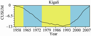

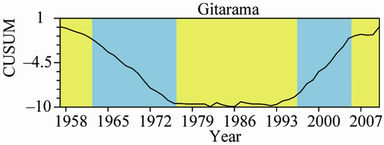
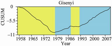

Figure 5. CUSUM chart for the mean annual maximum temperature for the five observatories.
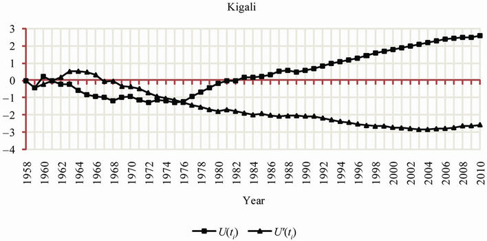
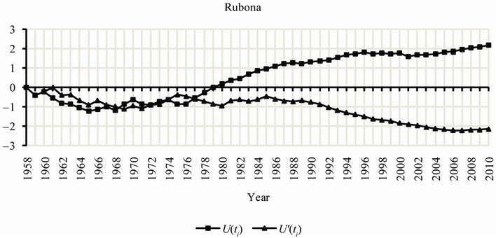
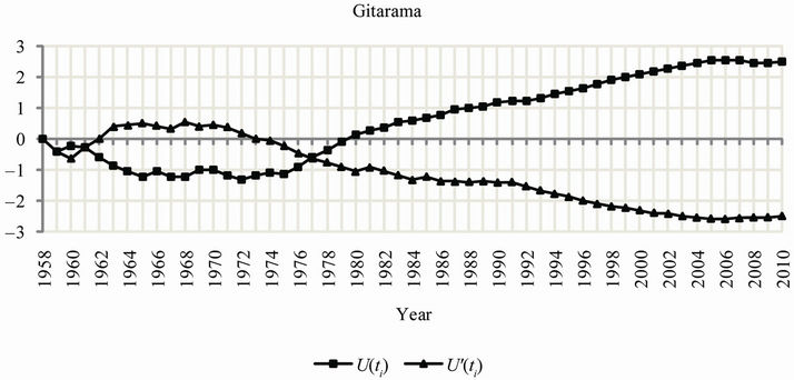
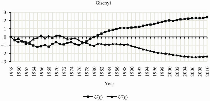
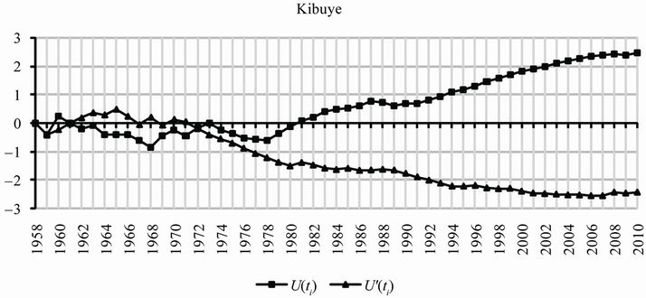
Figure 6. Trends of mean annual temperature (1958-2010) at the five observatories.
period 1958-2010 have been compared to trends of Global air temperature anomalies for the period 1958-2010 as it is shown in Figure 8. Results indicate that the trends observed in the increasing of temperature are roughly similar. The observed warming is most likely explained by the growing population accompanied by the increasing emission of green house gases, and the escalating urbanization and industrialization the country has experienced during the last decades, especially the capital City Kigali, during the last decades.
5. Conclusion
Long term time series of annual mean temperature has been compiled and analyzed. The data set has been carefully quality controlled and passed an intensive homogeneity assessment. Long term time series have been adjusted for further statistical analysis. There is a clear indication that climate change has occurred in Rwanda. Statistically significant abrupt changes and trends have been detected. The major change point in the annual mean temperature occurred around 1977 for all observa-
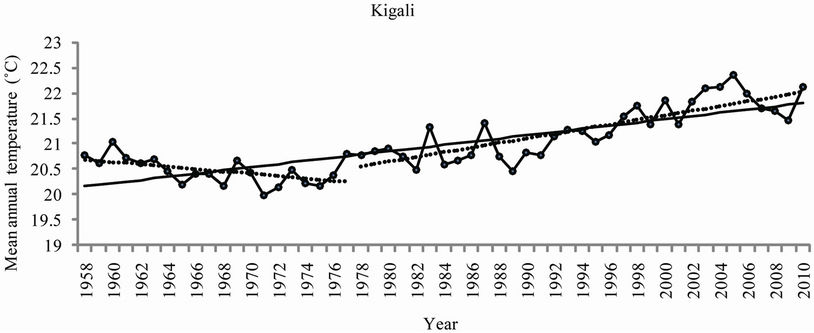
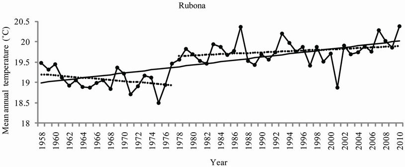

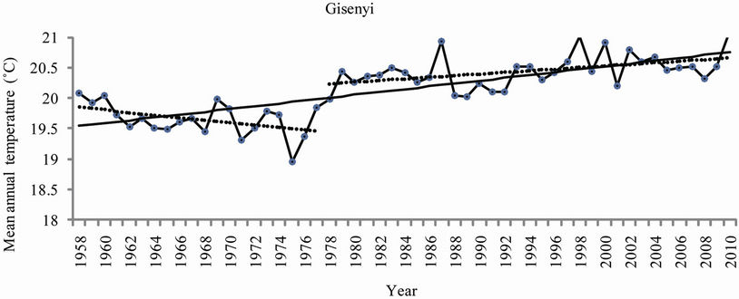

Figure 7. Annual trends of mean annual temperature (1958-2010) at the five observatories.
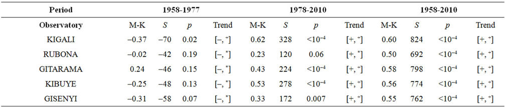
Table 4. Mann-Kendall statistics for the five observatories. M-K, S and p are respectively the Kendall’s tau statistic, the Kendall score and the two-sided p-value. (+ and – indicate respectively positive trend and negative trend, +, * indicate respectively significant and not significant at confidence level α = 0.05).
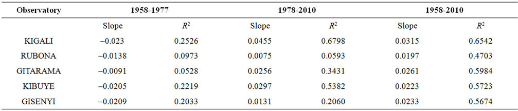
Table 5. Slope (˚C/year) and regression coefficient R2 for the trends of mean annual temperature for the five observatories corresponding to the periods 1958-1977, 1978-2010 and 1958-2010.

Figure 8. Global air temperature 2010 anomalies + 0.47˚C (left) compared to Rwanda air temperature 2010 anomalies + 0.97˚C (right) for the period 1958-2010. Global data are extracted from Phil Jones http://www.cru.uea.ac.uk/cru/info/warming/.
tories. The analysis of the annual mean temperature showed a not very significant cooling trend during the period ranging from 1958 to 1977 for all observatories. A significant warming trend was furthermore observed for the period after the year 1977 for all observatories where Kigali, the Capital of Rwanda, presented the highest values of the slope (0.0455/year) with high value of coefficient of determination (R2 = 0.6798), the Kendall’s tau statistic (M-K = 0.62), the Kendall Score (S = 328) with a two-sided p-value far less than the confidence level α of 5%). The observed warming is most likely explained by the growing population accompanied by the increasing emission of green house gases, and the escalating urbanization and industrialization the country has experienced, especially the capital City Kigali, during the last decades.
6. Acknowledgements
The author is grateful to the National Meteorological Service of the Ministry of Infrastructure (Rwanda), for providing relevant information for this article. The present study has been supported by the Research Commission of the National University of Rwanda (NUR) through a partnership with the Swedish International Agency SIDA/SAREC.
REFERENCES
- IPCC, “Climate Change 2007: Synthesis Report,” In: R. K. Pachauri and A. Reisinger, Eds., Contribution of Working Groups I, II and III to the Fourth Assessment Report of the Intergovernmental Panel on Climate Change (IPCC), Cambridge University Press, Cambridge, 2007.
- IPCC, “Climate Change 2007: The Physical Science Basis,” In: S. Solomon, D. Qin, M. Manning, Z. Chen, M. Marquis, K. B. Averyt, M. Tignor and H. L. Miller, Eds., Contribution of Working Group I to the Fourth Assessment Report of the Intergovernmental Panel on Climate Change (IPCC), Cambridge University Press, Cambridge, 2007.
- IPCC, “Climate Change 2007: Impacts, Adaptation and Vulnerability,” In: M. L. Parry, O. F. Canziani, J. P. Palutikof, P. J. van der Linden and C. E. Hanson, Eds., Contribution of Working Group II to the Fourth Assessment Report of the Intergovernmental Panel on Climate Change (IPCC), Cambridge University Press, Cambridge, 2007.
- IPCC, “Climate Change 2007: Mitigation of Climate Change,” In: B. Metz, O. R. Davidson, P. R. Bosch, R. Dave and L. A. Meyer, Eds., Contribution of Working Group III to the Fourth Assessment Report of the Intergovernmental Panel on Climate Change (IPCC), Cambridge University Press, Cambridge, 2007.
- R. Joeri, H. William, H. L. Jason, D. P. van Vuuren, R. Keywan, B. Matthews, H. Tatsuya, J. Kejun and M. Malte, “Emission Pathways Consistent with a 2˚C Global Temperature Limit,” Nature Climate Change, Vol. 1, No. 1, 2011, pp. 413-418. doi:10.1038/nclimate1258
- R. W. Spencer, “The Discovery of Global Warming,” American Institute of Physics, Harvard University Press, 2008. http://www.aip.org/history/climate/co2.htm
- Joint Science Academies’ Statement: Global Response to Climate Change, 2005. http://nationalacademies.org/onpi/06072005.pdf
- D. E. Parker and L. V. Alexander, “Global and Regional Climate in 2001,” Weather, Vol. 57, No. 9, 2002, pp. 328-340. doi:10.1256/00431650260283505
- P. Brohan, J. J. Kennedy, I. Harris, S. F. B. Tett and P. D. Jones, “Uncertainty Estimates in Regional and Global Observed Temperature Changes: A New Dataset from 1850,” Journal of Geophysical Research, Vol. 111, 2006. D12106. doi:10.1029/2005JD006548
- P. D. Jones and A. Moberg, “Hemispheric and LargeScale Surface Air Temperature Variations: An Extensive Revision and Update to 2001,” Journal of Climate, Vol. 16, 2003, pp. 206-223. doi:10.1175/1520-0442(2003)016<0206:HALSSA>2.0.CO;2
- W. Soon, S. Baliunas, E. S. Posmentier and P. Okeke, “Variations of Solar Coronal Hole Area and Terrestrial Lower Tropospheric Air Temperature from 1979 to Mid-1998: Astronomical Forcing of Change in Earth’s Climate,” New Astron, Vol. 4, No. 8, 2000, pp. 563-579. doi:10.1016/S1384-1076(00)00002-6
- T. Landscheidt, “Solar Wind near Earth: Indicator of Variations in Global Temperature,” Proceedings of the 1st Solar and Space Weather Euroconference on the Solar Cycle and Terrestrial Climate, Tenerife, 2000, pp. 497-500.
- K. Y. Vinnikov and N. C. Grody, “Global Warming Trend of Mean Troposphere Temperature Observed by Satellites,” Science, Vol. 302, No. 5643, 2003, pp. 269- 272. doi:10.1126/science.1087910
- P. D. Jones, D. E. Parker, T. J. Osborn and K. R. Briffa, “Global and Hemispheric Temperature Anomalies-Land and Marine Instrumental Records,” Trends: A Compendium of Data on Global Change, 2011. http://cdiac.ornl.gov/trends/temp/jonescru/jones.html
- S. Christoph Schär, L. V. Pier, L. Daniel, F. Christoph, H. Christian, A. L. Mark and A. Christof, “The Role of Increasing Temperature Variability in European Summer Heatwaves,” Nature, Vol. 427, 2004, pp. 332-336. doi:10.1038/nature02300
- N. W. Arnell, “The Effect of Climate Change on Hydrological Regimes in Europe: A Continental Per-Spective,” Global Environmental Change, Vol. 9, No. 1, 1999, pp. 5-23. doi:10.1016/S0959-3780(98)00015-6
- A. M. Aesawy and H. M. Hasanean, “Annual and Seasonal Climatic Analysis of Surface Air Temperature Variations at Six Southern Mediterranean Observatories,” Theoretical and Applied Climatology, Vol. 61, 1998, pp. 55-68. doi:10.1007/s007040050051
- K. Mikdat, “Trends in Surface Air Temperature Data over Turkey,” International Journal of Climatology, Vol. 17, 1997, pp. 511-520. doi:doi:10.1002/(SICI)1097-0088(199704)17:5<511::AID-JOC130>3.0.CO;2-0
- R. W. Hinggis, A. Leetmaa and V. E. Kousky, “Relationships between Climate Variability and Winter Temperature Extreme in the United States,” Journal of Climate, Vol. 15, 2002, pp. 1555-1572. doi:10.1175/1520-0442(2002)015<1555:RBCVAW>2.0.CO;2
- D. R. Easterling, H. F. Diaz, A. V. Douglas, W. D. Hogg, K. E. Kunkel, J. C. Rogers and J. F. Wilkinson, “LongTerm Observations for Monitoring Extremes in the Americas,” Climatic Change, Vol. 42, 1999, pp. 285-308. doi:10.1023/A:1005484820026
- D. P. Lettenmaier, E. F. Wood and J. R. Wallis, “HydroClimatological Trends in the Continental United States 1948-1988,” Journal of Climate, Vol. 7, 1994, pp. 586- 607. doi:10.1175/1520-0442(1994)007<0586:HCTITC>2.0.CO;2
- M. S. Mahmoud Smadi and Z. Ahmed, “A Sudden Change in Rainfall Characteristics in Amman, Jordan during the Mid 1950s,” American Journal of Environmental Sciences, Vol. 2, No. 3, 2006, pp. 84-91. doi:10.3844/ajessp.2006.84.91
- S. Al-Fahed, O. Al-Hawaj and W. Chakroun, “The Recent Air Temperature Rise in Kuwait,” Renewable Energy, Vol. 12, No. 1, 1997, pp. 83-90. doi:10.1016/S0960-1481(97)00015-3
- N. A. Elagib and A. S. Abdu, “Climate Variability and Aridity in Bahrain,” Journal of Arid Environmental, Vol. 36, No. 3, 1997, pp. 405-419. doi:10.1006/jare.1996.0237
- K. Mikdat and S. Levent, “Trends of Growing DegreeDays in Turkey,” Water, Air and Soil Pollution, Vol. 126, No. 1-2, 2000, pp. 83-96. doi:10.1023/A:1005299619084
- N. I. Obot, M. A. C. Chendo, S. O. Udo and I. O. Ewona, “Evaluation of Rainfall Trends in Nigeria for 30 Years (1978-2007),” International Journal of the Physical Sciences, Vol. 5, No. 14, 2010, pp. 2217-2222.
- E. Aguilar, et al., “Changes in Temperature and Precipitation Extremes in Western Central Africa, Guinea Conakry, and Zimbabwe, 1955-2006,” Journal of Geophysical Research, Vol. 11, 2009, D02115. doi:10.1029/2008JD011010
- P. Heiko, B. Kai, G. Robin, P. Ralf and J. Daniela, “Regional Climate Change in Tropical and Northern Africa Due to Greenhouse Forcing and Land Use Changes,” Journal of Climate, Vol. 22, 2009, pp. 114-132. doi:10.1175/2008JCLI2390.1
- M. New, et al., “Evidence of Trends in Daily Climate Extremes over Southern and West Africa,” Journal of Geophysical Research, Vol. 11, 2006, pp. 1-11. doi:10.1029/2005JD006289
- A. C. Kruger, “Observed Trends in Daily Precipitations Indices in South Africa: 1919-2004,” International Journal of Climatology, Vol. 26, 2006, pp. 2275-2285. doi:10.1002/joc.1368
- S. E. Nicholson, “Climatic and Environmental Change in Africa during the Last Two Centuries,” Climate Research, Vol. 17, 2001, pp. 123-144. doi:10.3354/cr017123
- M. R. Hulme, T. Doherty Ngara and D. Lister, “African Climate Change: 1900-2100,” Climate Research, Vol. 17, 2001, pp. 145-168. doi:10.3354/cr017145
- S. E. Nicholson, “The Nature of Rainfall Variability over Africa on Time Scales of Decades to Millennia,” Global and Planetary Change, Vol. 26, 2000, pp. 137-158. doi:10.1016/S0921-8181(00)00040-0
- S. M. King’uyu, L. A. Ogallo and E. K. Anyamba, “Recent Trends on Minimum and Maximum Surface Temperatures over Eastern Africa,” Journal of Climate, Vol. 13, No. 13, 2000, pp. 2876-2886. doi:10.1175/1520-0442(2000)013<2876:RTOMAM>2.0.CO;2
- J. M. Collins, “Temperature Variability over Africa,” Journal of Climate, Vol. 24, No. 14, 2011, pp. 3649-3666. doi:10.1175/2011JCLI3753.1
- S. E. Nicholson and J. Kim, “The Relationship of the El Niño Southern Oscillation to African Rainfall,” International Journal of Climatology, Vol. 17, 1997, pp. 117-135. doi:10.1002/(SICI)1097-0088(199702)17:2<117::AID-JOC84>3.0.CO;2-O
- R. A. Pielke, “Land Use and Climate Change,” Science, Vol. 310, No. 5754, 2005, pp. 1625-1626. doi:10.1126/science.1120529
- E. Kalnay and M. Cai, “Impact of Urbanization and Land-Use Change on Climate,” Nature, Vol. 423, 2003, pp. 528-531. doi:10.1038/nature01675
- P. I. Figuerola and A. N. Mazzeo, “Urban-Rural Temperature Differences in Buenos Aires,” International Journal of Climatology, Vol. 18, No. 15, 1998, pp. 1709- 1723. doi:10.1002/(SICI)1097-0088(199812)18:15<1709::AID-JOC338>3.0.CO;2-I
- R. Bohn, “Urban Bias in Temperature Time Series—A Case Study for the City of Vienna, Austria,” Climatic Change, Vol. 38, No. 1, 1998, pp. 113-128. doi:10.1023/A:1005338514333
- M. Tayanc and H. Toros, “Urbanization Effects on Regional Climate Change in the Case of Four Large Cities of Turkey,” Climatic Change, Vol. 35, No. 4, 1997, pp. 501-524. doi:10.1023/A:1005357915441
- Y. R. Adebayo, “A Note on the Effect of Urbanization on Temperature in Ibadan,” Journal of Climatology, Vol. 7, No. 2, 1987, pp. 185-192. doi:10.1002/joc.3370070209
- R. C. Robert Jr. and W. B. Sandra, “The Impact of Rapid Urbanization on Pan Evaporation in Phoenix, Arizona,” Journal of Climatology, Vol. 7, No. 6, 1987, pp. 593-597. doi:10.1002/joc.3370070607
- E. Aguilar, I. Auer, M. Brunet, T. Peterson and J. Wieringa, “Guidelines on Climate Metadata and Homogenization,” WMO TD. No. 1186 (WCDMP2), World Meteorological Organization, Geneva, 2003.
- W. P. He, G. L. Feng, Q. Wu, T. He, S. Q. Wan and J. F. Chou, “A New Method for Abrupt Dynamic Change Detection of Correlated Time Series,” International Journal of Climatology, 2011. doi:10.1002/joc.2367
- M. J. Menne and C. N. Williams Jr., “Homogenization of Temperature Series via Pairwise Comparisons,” Journal of Climate, Vol. 22, No. 7, 2009, pp. 1700-1717. doi:10.1175/2008JCLI2263.1
- M. Brunet, et al., “Temporal and Spatial Temperature Variability and Change over Spain during 1850-2005,” Journal of Geophysical Research, Vol. 112, 2007, D12117. doi:10.1029/2006JD008249
- P. M. Della-Marta and H. Wanner, “A Method of Homogenizing the Extremes and Mean of Daily Temperature Measurements,” Journal of Climate, Vol. 19, 2006, pp. 4179-4197. doi:10.1175/JCLI3855.1
- C. Serra, A. Burgueno and X. Lana, “Analysis of Maximum and Minimum Daily Temperatures Recorded at Fabra Observatory (Barcelona, Ne Spain) in the Period 1917-1998,” International Journal of Climatology, Vol. 21, 2001, pp. 617-636. doi:10.1002/joc.633
- T. C. Peterson, D. R. Easterling, T. R. Karl, et al., “Homogeneity Adjustments of in Situ Atmospheric Climate Data: A Review,” International Journal of Climatology, Vol. 18, No. 13, 1998, pp. 1493-1517. doi:10.1002/(SICI)1097-0088(19981115)18:13<1493::AID-JOC329>3.0.CO;2-T
- T. R. Karl and C. N. Williams Jr., “An Approach to Adjusting Climatological Time Series for Discontinuous Inhomogeneities,” Journal of Climate & Applied Meteorology, Vol. 26, No. 12, 1987, pp. 1744-1763. doi:10.1175/1520-0450(1987)026<1744:AATACT>2.0.CO;2
- H. Alexanderson, “A Homogeneity Test Applied to Precipitation Data,” Journal of Climatology, Vol. 6, 1986, pp. 661-675. doi:10.1002/joc.3370060607
- T. A. Buishan, “Some Methods for Testing the Homogeneity of Rainfall Records,” Journal of Hydrology, Vol. 58, 1982, pp. 11-27. doi:10.1016/0022-1694(82)90066-X
- W. Taylor, “Change-Point Analysis: A Powerful New Tool for Detecting Changes,” Taylor Enterprises, Libertyville, 2000. http://www.variation.com/cpa/tech/changepoint
- W. Taylor, “Change-Point Analyzer 2.3 Software Package,” Taylor Enterprises, Libertyville, 2000. http://www.variation.com/cpa/tech/changepoint
- A. C. Davison and D. V. Hinkley, “Bootstrap Methods and Their Application,” Cambridge University Press, Cambridge, 1997.
- Y. Sheng and P. Paul, “A Comparison of the Power of the t Test, Mann-Kendall and Bootstrap Tests for Trend Detection”, Hydrological Sciences Journal, Vol. 49, No. 1, 2004, pp. 21-37. doi:10.1623/hysj.49.1.21.53996
- R. Sneyers, “On the Statistical Analysis of Series of Observations,” WMO Technical Note 143, WMO No. 415, TP-103, World Meteorological Organization, Geneva, 1990.
- A. John, “Fisher and Regression,” Statistical Science, Vol. 20, No. 4, 2005, pp. 401-417. doi:10.1214/088342305000000331
- [61] M. G. Kendall and J. D. Gibbons, “Rank Correlation Methods,” 4th Edition, Griffin, London, 1990.