Journal of Water Resource and Protection
Vol. 2 No. 3 (2010) , Article ID: 1499 , 15 pages DOI:10.4236/jwarp.2010.23031
Simulation of Runoff and Sediment Yield for a Himalayan Watershed Using SWAT Model
1National Institute of Hydrology, Roorkee, India
2Alternate Hydro-Energy Centre, I IT, Roorkee, India
E-mail: sjain@nih.ernet.in
Received October 12, 2009; revised December 7, 2009; accepted January 25, 2010
Keywords: AVSWATX, Calibration, Validation, Image Processing, Remote Sensing, GIS, Runoff, Sediment Yield
ABSTRACT
Watershed is considered to be the ideal unit for management of the natural resources. Extraction of watershed parameters using Remote Sensing and Geographical Information System (GIS) and use of mathematical models is the current trend for hydrologic evaluation of watersheds. The Soil and Water Assessment Tool (SWAT) having an interface with ArcView GIS software (AVSWAT2000/X) was selected for the estimation of runoff and sediment yield from an area of Suni to Kasol, an intermediate watershed of Satluj river, located in Western Himalayan region. The model was calibrated for the years 1993 & 1994 and validated with the observed runoff and sediment yield for the years 1995, 1996 and 1997. The performance of the model was evaluated using statistical and graphical methods to assess the capability of the model in simulating the runoff and sediment yield from the study area. The coefficient of determination (R2) for the daily and monthly runoff was obtained as 0.53 and 0.90 respectively for the calibration period and 0.33 and 0.62 respectively for the validation period. The R2 value in estimating the daily and monthly sediment yield during calibration was computed as 0.33 and 0.38 respectively. The R2 for daily and monthly sediment yield values for 1995 to 1997 was observed to be 0.26 and 0.47.
1. Introduction
A Watershed is a hydrologic unit which produces water as an end product by interaction of precipitation and the land surface. The quantity and quality of water produced by the watershed are an index of amount and intensity of precipitation and the nature of watershed management. In some watersheds the aim may be to harvest maximum total quantity of water throughout the year for irrigation and drinking purpose. In another watershed the objectives may be to reduce the peak rate of runoff for minimizing soil erosion and sediment yield or to increase ground water recharge. Hence, the modeling of runoff, soil erosion and sediment yield are essential for sustainable development. Further, the reliable estimates of the various hydrological parameters including runoff and sediment yield for remote and inaccessible areas are tedious and time consuming by conventional methods. So it is desirable that some suitable methods and techniques are used/ evolved for quantifying the hydrological parameters from all parts of the watersheds. Use of mathematical models for hydrologic evaluation of watersheds is the current trend and extraction of watershed parameters using remote sensing and geographical information system (GIS) in high speed computers are the aiding tools and techniques for it.
The Satluj river basin as a whole receives a good amount of rainfall throughout the year, which flows through the Western Himalayan region. Apart from the hill topography, faulty cultivation practices and deforestation within the basin result in huge loss of productive soil and water as runoff. There is an urgent need for developing integrated watershed management plan based on hydrological simulation studies using suitable modeling approach. Considering hydrological behaviour of the basin and applicability of the existing models for the solutions of aforesaid problems, the current study was undertaken with the application of SWAT 2000 in integration with remote sensing and GIS to estimate the surface runoff and sediment yield of an intermediate watershed of Satluj river (Suni to Kasol). The AVSWAT is a preprocessor and as well as a user interface to SWAT model. The application of AVSWAT2000/X in the present study provided the capabilities to stream line GIS processes tailored towards hydrologic modeling and to automate data entry communication and editing environment between GIS and the hydrologic model. The time series data on rainfall, runoff and sediment yield were available at the gauging station of the catchment and these were used to calibrate and validate the SWAT model and to assess its applicability in simulating runoff and sediment yield from the intermediate watershed in the Himalayan region.
2. The Study Area
The data of an intermediate watershed of Satluj river was used for assessment of runoff and sediment yield in the present study. The study watershed (Figure 1) lying between Suni to Kasol in the state of Himachal Pradesh, India is located between latitudes 31˚ 5` to 31˚ 30` N and longitudes 76˚ 50` to 77˚15` E. The watershed covers an area of about 681.5 sq km with an elevation between 600 to 3200 m above mean sea level (msl). The Satluj River flows through the Western Himalayan region. The Western Himalayas cover the hilly areas of JammuKashmir, Himachal Pradesh and Uttarakhand states in India. Two important river systems originating from the Western Himalayan region are 1) Indus system consisting of Indus, Jhelum, Chenab, Ravi, Beas and Satluj rivers, and 2) Ganga system consisting of Yamuna, Ramganga, Sarda, and Karnali rivers. These rivers are fed by snowmelt and rainfall during the summer and by groundwater flow during the winter.
3. Swat Model
The SWAT (Soil and Water Assessment Tool) is one of the most recent models developed jointly by the United States Department of Agriculture - Agricultural Research Services (USDA-ARS) and Agricultural Experiment Station in Temple, Texas [1]. It is a physically based, continuous time, long-term simulation, lumped parameter, deterministic, and originated from agricultural models. The computational components of SWAT can be placed into eight major divisions: hydrology, weather, sedimentation, soil temperature, crop growth, nutrients, pesticides, and agricultural management. The SWAT model uses physically based inputs such as weather variables, soil properties, topography, and vegetation and land management practices occurring in the catchment. The physical processes associated with water flow, sediment transport, crop growth, nutrient cycling, etc. are directly modeled by SWAT [2,3]. Some of the advantages of the model include: modeling of ungauged
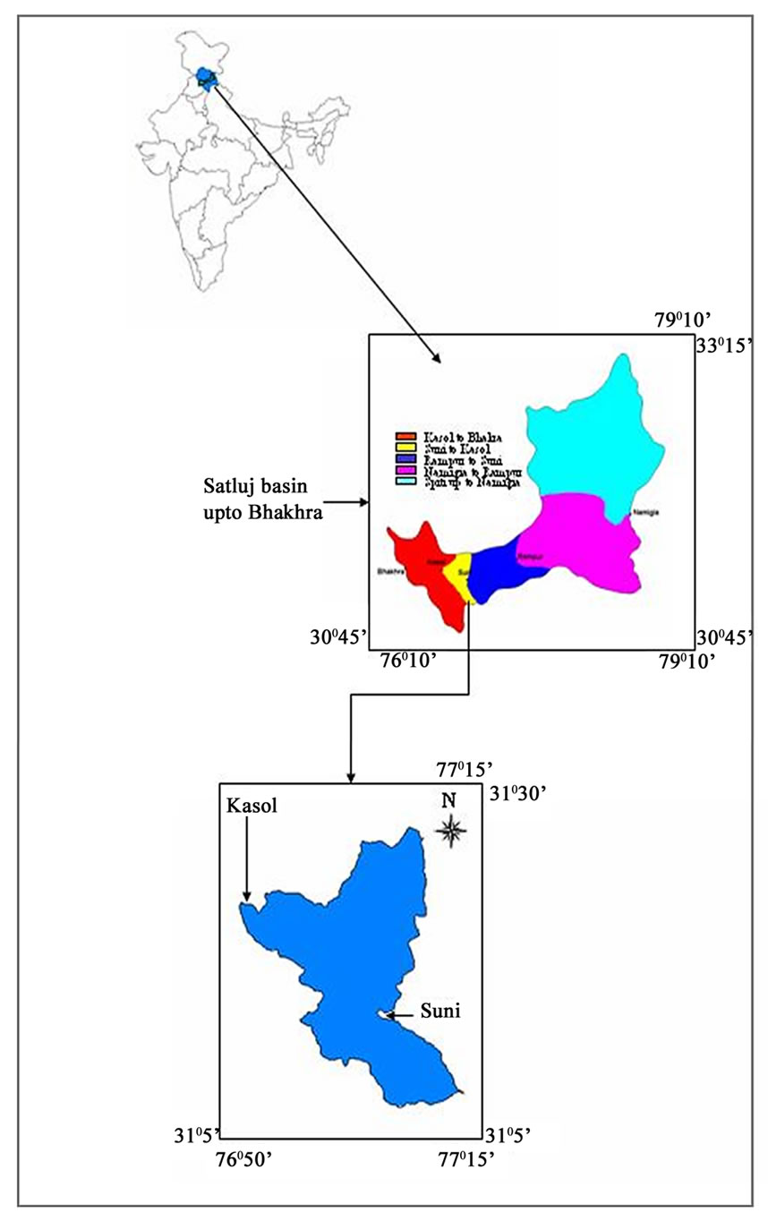
Figure 1. Study area between Suni to Kasol.
catchments, prediction of relative impacts of scenarios (alternative input data) such as changes in management practices, climate and vegetation on water quality, quantity or other variables. SWAT has a weather simulation model also that generates daily data for rainfall, solar radiation, relative humidity, wind speed and temperature from the average monthly variables of these data. This provides a useful tool to fill in missing daily data in the observed records. The hydrologic cycle as simulated by SWAT is based on the water balance equation:
where, SWt is the final soil water content (mm H2O), SWo is the initial soil water content (mm H2O), t is time in days, Rday is amount of precipitation on day i (mm H2O), Qsurf is the amount of surface runoff on day i (mm H2O), Ea is the amount of evapotranspiration on day i (mm H2O), wseep is the amount of percolation and bypass exiting the soil profile bottom on day i (mm H2O), Qgw is the amount of return flow on day i (mm H2O).
In SWAT, a basin is delineated into sub-basins, which are then further subdivided into hydrologic response units (HRUs). HRUs consist of homogeneous land use and soil type (also, management characteristics) and based on two options in SWAT, they may either represent different parts of the sub-basin or sub-basin area with a dominant land use or soil type (also, management characteristics). With this semi-distributed (sub-basins) set-up, SWAT is attractive for its computational efficiency as it offers some compromise between the constraints imposed by the other model types such as lumped, conceptual or fully distributed, physically based models. A full model description and operation is presented in Neitsch et al. [4,5]. SWAT uses hourly and daily time steps to calculate surface runoff. The Green and Ampt equation is used for hourly and an empirical SCS curve number (CN) method is used for the daily computation.
Spruill et al. [6] evaluated the SWAT model and parameter sensitivities were determined while modeling daily streamflow in a small central Kentucky watershed comprising an area of 5.5 km2 over a two year period. Streamflow data from 1996 were used to calibrate the model and streamflow data from 1995 were used for evaluation. The model accurately predicted the trends in daily streamflow during this period. The Nash-Sutcliffe [7] R2 for monthly total flow was 0.58 for 1995 and 0.89 for 1996 whereas for daily flows it was observed to be 0.04 and 0.19. The monthly total tends to smooth the data which in turn increases the R2 value. Overall the results indicated that SWAT model can be an effective tool for describing monthly runoff from small watersheds.
Fohrer et al. [8] applied three GIS based models from the field of agricultural economy (ProLand), ecology (YELL) and hydrology (SWAT-G) in a mountainous meso-scale watershed of Aar, Germany covering an area of 59.8 km2 with the objective of developing a multidisciplinary approach for integrated river basin management. For the SWAT–G model daily stream flow were predicted. The model was calibrated and validated followed by model efficiency using Nash and Sutcliffe test. In general the predicted streamflow showed a satisfying correlation for the actual landuse with the observed data.
Francos et al. [9] applied the SWAT model to the Kerava watershed (South of Finland), covering an area of 400 km2. The temporal series comprised temperature and precipitation records for a number of meteorological stations, water flows and nitrogen and phosphorus loads at the river outlets. The model was adapted to the specific conditions of the catchment by adding a weather generator and a snowmelt submodel calibrated for Finland. Calibration was made against water flows, nitrate and total phosphorus concentrations at the basin outlet. Simulations were carried out and simulated results were compared with daily measured series and monthly averages. In order to measure the accuracy obtained, Nash and Suttcliffe efficiency coefficient was employed which indicated a good agreement between measured and predicted values.
Eckhartd and Arnold [10] outlined the strategy of imposing the constraints on the parameters to limit the number of interdependently calibrated values of SWAT. Subsequently an automatic calibration of the version SWAT-G of the SWAT model with a stochastic global optimization algorithm and Shuffled Complex Evolution algorithm is presented for a mesoscale catchment.
Tripathi et al. [11] applied the SWAT model for Nagwan watershed (92.46km2) with the objective of identifying and prioritizing of critical sub-watersheds to develop an effective management plan. Daily rainfall, runoff and sediment yield data of 7 years (1992-1998) were used for the study. Apart from hydro-meteorological data, topographical map, soil map, land resource map and satellite imageries for the study area were also used. The model was verified for the monsoon season on daily basis for the year 1997 and monthly basis for the years 1992-1998 for both surface runoff and sediment yield.
Singh et al. [12] made a comparative study for the Iroquois river watershed covering an area of 2137 sq. miles with the objectives to assess the suitability of two watershed scale hydrologic and water quality simulation models namely HSPF and AVSWAT 2000. Based on the completeness of meteorological data, calibration and validation of the hydrological components were carried out for both the models. Time series plots as well as statistical measures such as Nash-Sutcliffe efficiency, coefficient of correlation and percent volume errors between observed and simulated streamflow values on both monthly and annual basis were used to verify the simulation abilities of the models.
The review indicated that SWAT is capable of simulating hydrological processes with reasonable accuracy and can be applied to large ungauged basin. Therefore, to test the capability of model in determining the effect of spatial variability of the watershed on runoff, AVSWAT 2000 with arcview interface was selected for the present study.
3. Methodology
3.1. Creation of Data Base
Digital elevation model (DEM) is one of the main inputs of SWAT Model. For preparation of DEM, the vector map with contour lines (from topographic maps) was converted to raster format (Grid) before the surface was interpolated. Grids are especially suited to representing geographic phenomena that vary continuously over space, and for performing spatial modeling and analysis of flows, trends, and surfaces such as hydrology. Raster data records spatial information in a regular grid or matrix organized as a set of rows and columns. The DEM of the study watershed is shown in Figure 2. The drainage map (Figure 3) was digitized using Survey of India toposheets at a scale of 1:50,000. The drainage map can be entered into AVSWAT as shape file and grid format.
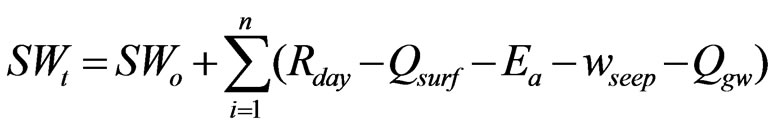
Landuse map is a critical input for SWAT model. Land use/land cover map was prepared using remote sensing data of Landsat ETM+. The classification of satellite data mainly follows two approaches i.e. supervised and unsupervised classification. The intent of the classification process is to categorize all pixels in a digital image into one of several land cover classes, or “themes”. This categorized data may then be used to produce thematic maps of the land cover present in an image. In the present study, the unsupervised classification method was used for preparation of the land use map (Figure 4). The various land use categories and their coverage in the study watershed are presented in Table 1.
Soil map of the study area was digitized using soil map of the National Bureau of Soil Survey and Land Use Planning (NBSS&LUP) at a scale of 1:50,000. Soil plays an important role in modeling various hydrological processes. In the AVSWATX model, various soil properties like soil texture, hydraulic conductivity, organic carbon content, bulk density, available water content are required to be analyzed to make an input in the model for simulation purpose. While carrying out the soil sampling, the soil map prepared by NBSS&LUP was used as a base map. The collected 26 soil samples were then analyzed in a standard soil laboratory. Based on the analysis it was observed that the soils in the study area were mostly clayey soils (Figure 5) and falls in the hydrologic soil group C & D.
A hydro-meteorological observation network was set up in the Satluj River basin by Bhakra Beas Management Board (BBMB), Nangal. The rainfall is observed at 10 stations namely Bhakra, Berthin, Kahu, Suni, Kasol, Rampur, Kalpa, Rackchham, Namgia and Kaza. In the present study, the rainfall data of Suni and Kasol stations were used. The flows were monitored at Suni and Kasol gauging sites on the main Satluj river. The gauge-discharge sites were monitored for 24 hours during the monsoon period to observe the high floods. The daily runoff and sediment load data of two stations namely Suni and Kasol were collected for the years 1993 through 1997. The processing of meteorological data was done statistically. The simulated daily weather data on maximum and minimum temperature, rainfall, wind speed and relative humidity at all the grid locations for 5 years representing the series approximating 1993 to 1997 time period were processed.
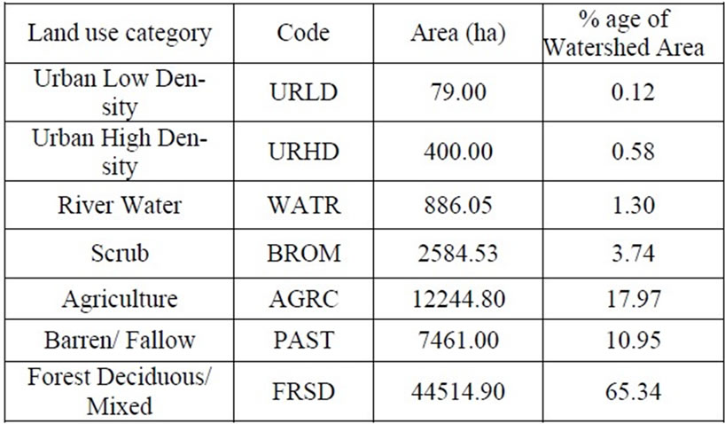
Table 1. Coverage of various land use categories in the study.
3.2. Model Set up
AVSWATX automatically delineates a watershed into sub-watersheds based on DEM and drainage network. After the DEM was imported in the model a masking polygon of the study area was created in Arc Info grid format and was loaded in the model in order to extract out only the area of interest. The critical source area or the minimum drainage area required to form the origin of a stream was taken as 2500 ha which formed 13 sub watersheds (Figure 6). The area delineated by the AVSWATX interface was found to be 68,134.23 ha against the manually delineated area of 68,170.28 ha. The error of calculation was found to be 0.02%.
The land use and soil map in Arcshape format were imported in the AVSWATX model. Both the maps were made to overlay to subdivide the study watershed into hydrologic response units (HRU) based on the land use and soil types. Subdividing the areas into hydrologic response units enables the model to reflect the evapotranspiration and other hydrologic conditions for different land cover/crops and soils. One of the main sets of input for simulating the hydrological processes in SWAT is climate data. Climate data input consists of precipitation, maximum and minimum temperature, wind speed, relative humidity and the weather generator (.dbf) file. The climate data for study periods were prepared in .dbf format and then imported in the SWAT model. After importing the climatic data, the next step was to set up a few additional inputs for running the SWAT model. These inputs were management data, soil-chemical data, manning’s roughness coefficient for overland flow and in-stream water quality parameters. These input files were set up and edited as per the requirement and objective of the study. In the management data file, runoff curve numbers for Indian conditions as well as those prescribed in SWAT user manual were adopted for different land use classes based on the land use type and hydrologic soil group (HSG). Finally the SWAT model was run to simulate the various hydrological components.
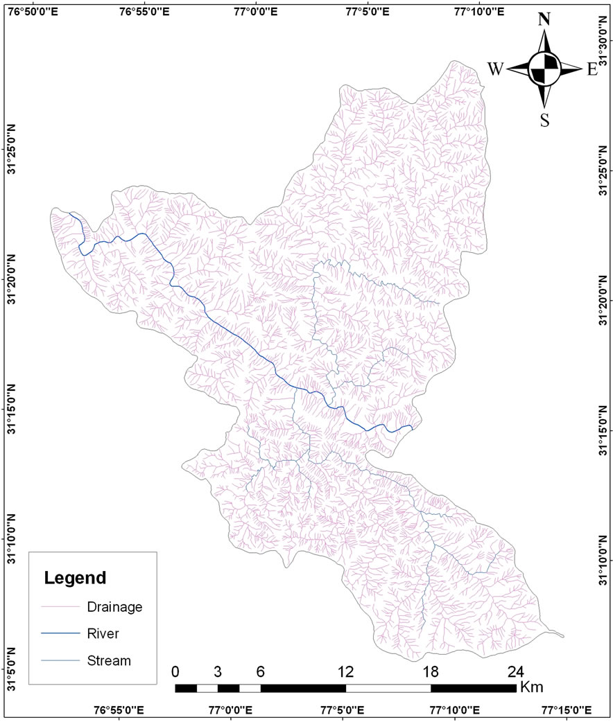
Figure 2. Digital elevation model of the study watershed.
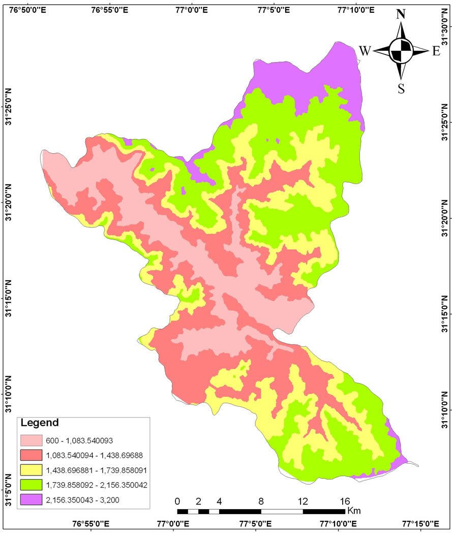
Figure 3. Drainage network in the study area.
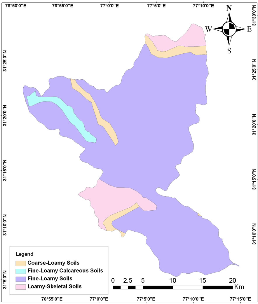
Figure 4. Landuse / landcover of the study area.
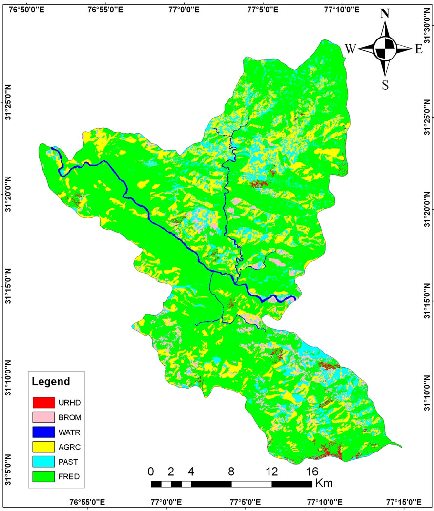
Figure 5. Soil texture map of the study area.
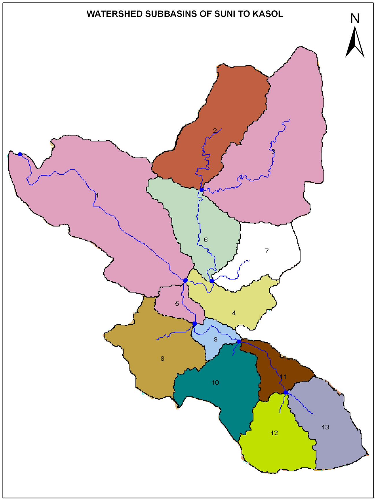
Figure 6. Delineation of sub-watersheds of the study area.
3.3. Performance Evaluation of the Model
Performance of the model was evaluated in order to assess how the model simulated values fitted with the observed values. Several statistical measures are available for evaluating the performance of a hydrologic model. These include coefficient of determination, relative error, standard error, volume error, coefficient of efficiency [13], among others. The coefficient of determination (R2) is one of the frequently used criteria and was employed in this study. R2 describes the proportion of the total variance in the measured data that can be explained by the model. It ranges from 0.0 to 1.0, with higher values indicating better agreement, and is given by,
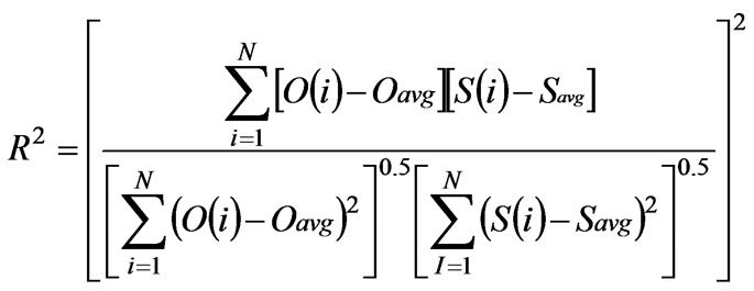
where, O(i) is the ith observed parameter, Oavg is the mean of the observed parameters, S(i) is the ith simulated parameter, Savg is the mean of model simulated parameters and N is the total number of events.
4. Results and Discussion
4.1. Model Calibration
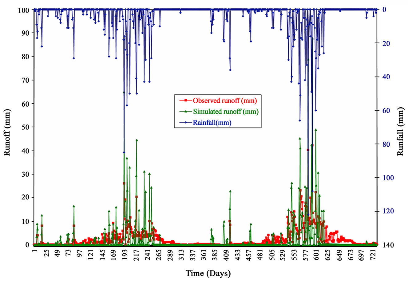
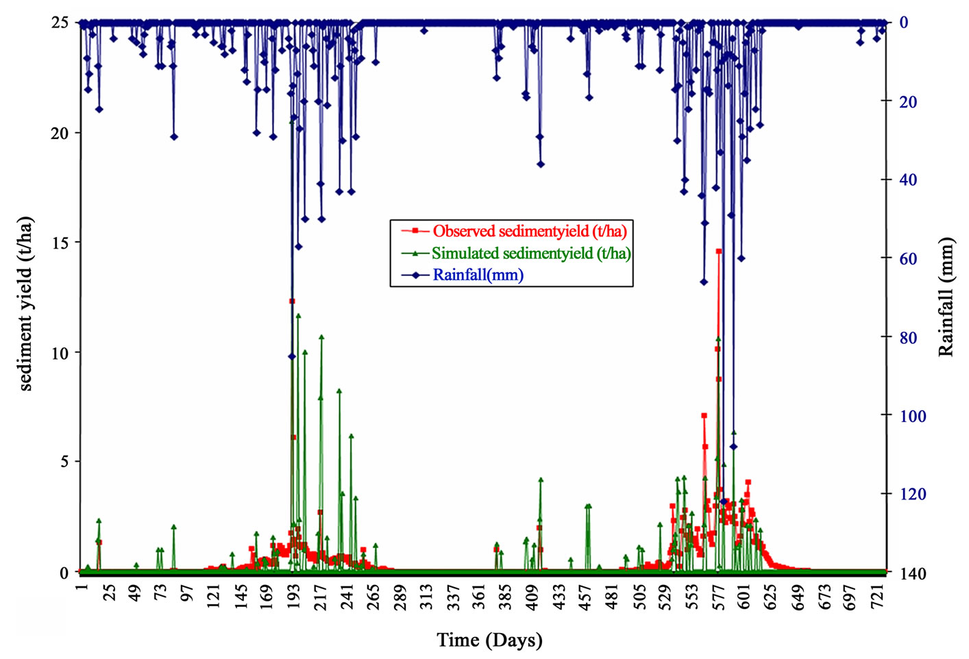
The AVSWATX model was calibrated using the daily data of runoff and sediment yield recorded at the outlet of the study watershed for the years 1993 & 1994. The model was calibrated using the values of parameters for available water content (AWC) and soil evaporation compensation factor (SECO) within the prescribed range of the model. Several simulation runs were applied to achieve the model calibration. The time series of the observed and simulated daily and monthly runoff (Figure 7(a), (b)) and daily and monthly sediment yield (Figure 8(a), (b)) for the calibration period were plotted for visual comparison. From these figures, it can be observed in general that the model
 (a)
(a)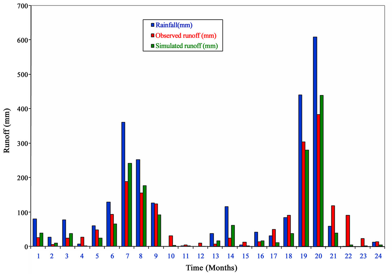 (b)
(b)
Figure 7. Comparison of observed and simulated. (a) daily runoff; (b) monthly runoff for the calibration period 1993-94.
 (a)
(a)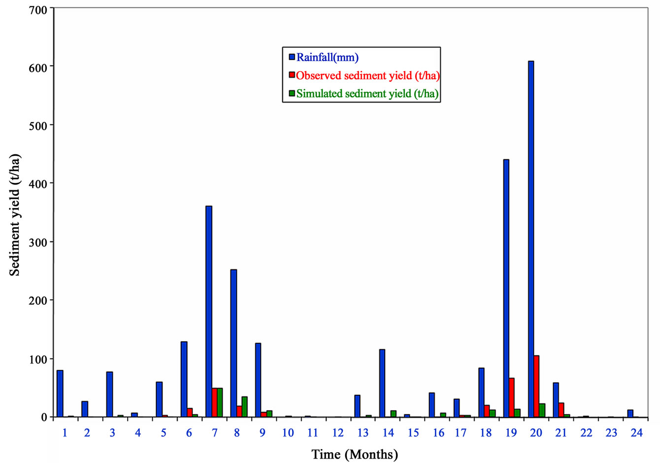 (b)
(b)
Figure 8. Comparison of observed and simulated. (a) daily sediment yield; (b) monthly sediment yield for the calibration period 1993-1994.
overestimated the peaks of both runoff and sediment yield in both the years of calibration. The total runoff computed by the model was, however, found to be 691.67 mm and 911.85 mm against the observed runoff of 729.82 mm and 1127.66 mm during 1993 and 1994 respectively. The sediment yield computed by the model during respective years was obtained as 114.72 t/ha and 106.27 t/ha against the observed sediment yield of 99.10 t/ha and 223.83 t/ha respectively. The observed and simulated values were plotted against each other in order to determine the goodness-of fit criterion of coefficient of determination (R2) both for runoff and sediment
 (a)
(a)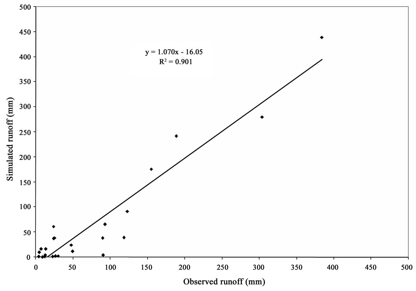 (b)
(b)
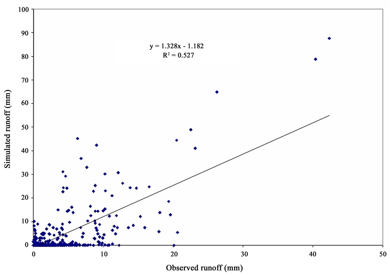
Figure 9. Goodness-of-fit for observed and simulated. (a) daily runoff; and (b) monthly runoff for the calibration period 1993-94.
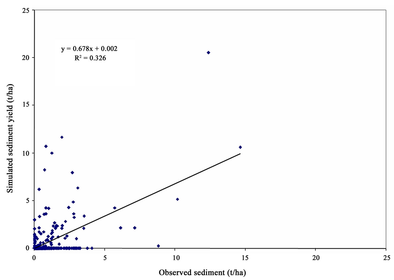
yield. The R2 value for daily and monthly values was obtained as 0.53 and 0.90 respectively for runoff (Figure 9(a), (b)) and 0.33 and 0.38 respectively for sediment yield (Figure 10(a), (b)). The analysis reveals that the monthly comparison showed a better correlation than the daily values. The poor correlation among daily values in the present study can be supported by the inferences of Peterson and Hamlett [14], Benaman et al. [15], Varanou et al. [16], Spruill et al. [6], and King et al. [17]. It was reported that SWAT’s daily flow predictions, in general, were not as good as monthly flow predictions. Simulated and observed daily flow comparisons yielded much lower Nash-Sutcliffe Coefficient (NSC) than monthly comparisons. The monthly totals tend to smooth the data, which in turn increases the NSC [6,18]. While simulating sediment loadings in the Cannonsville Reservoir watershed (1,178 km2) in New York, Benaman et al. [15] noted that the model generally simulated watershed response on sediment, but it grossly under predicted sediment yields during high flow months. In the present study, the error in simulation may also be attributed to some extent perhaps to the unreliable observed data. Another reason could be the number of delineated sub-watersheds. It is reported that watershed subdivision has an effect on the sediment load [19].
 (a)
(a)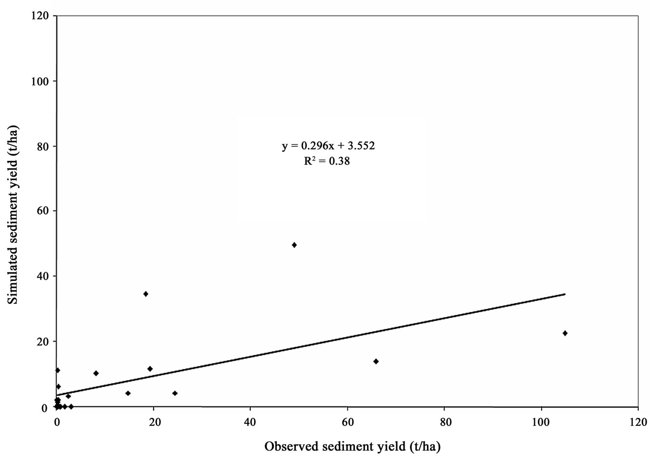 (b)
(b)
Figure 10. Goodness-of-fit for observed and simulated. (a) daily sediment yield; (b) monthly sediment yield for the calibration period 1993-94.
4.2. Model Validation
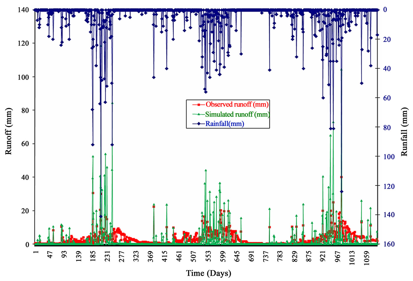
The model validation was carried out for daily and monthly surface runoff and sediment yield for the years 1995 to 1997. A graphical comparison of the observed and simulated daily and monthly flows (Figure 11(a), (b)) show that the peaks of the surface runoff were overestimated in most of the events. During the years 1995,
 (a)
(a)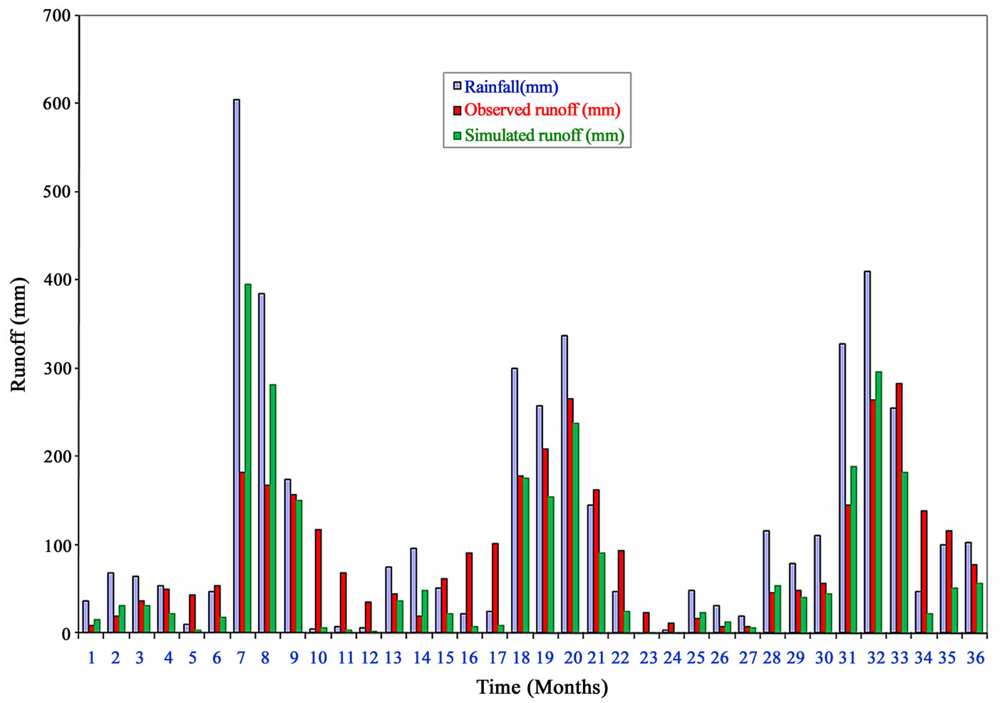 (b)
(b)
Figure 11. Comparison of observed and simulated (a) daily runoff, and (b) monthly runoff for the validation period 1995-97.
 (a)
(a)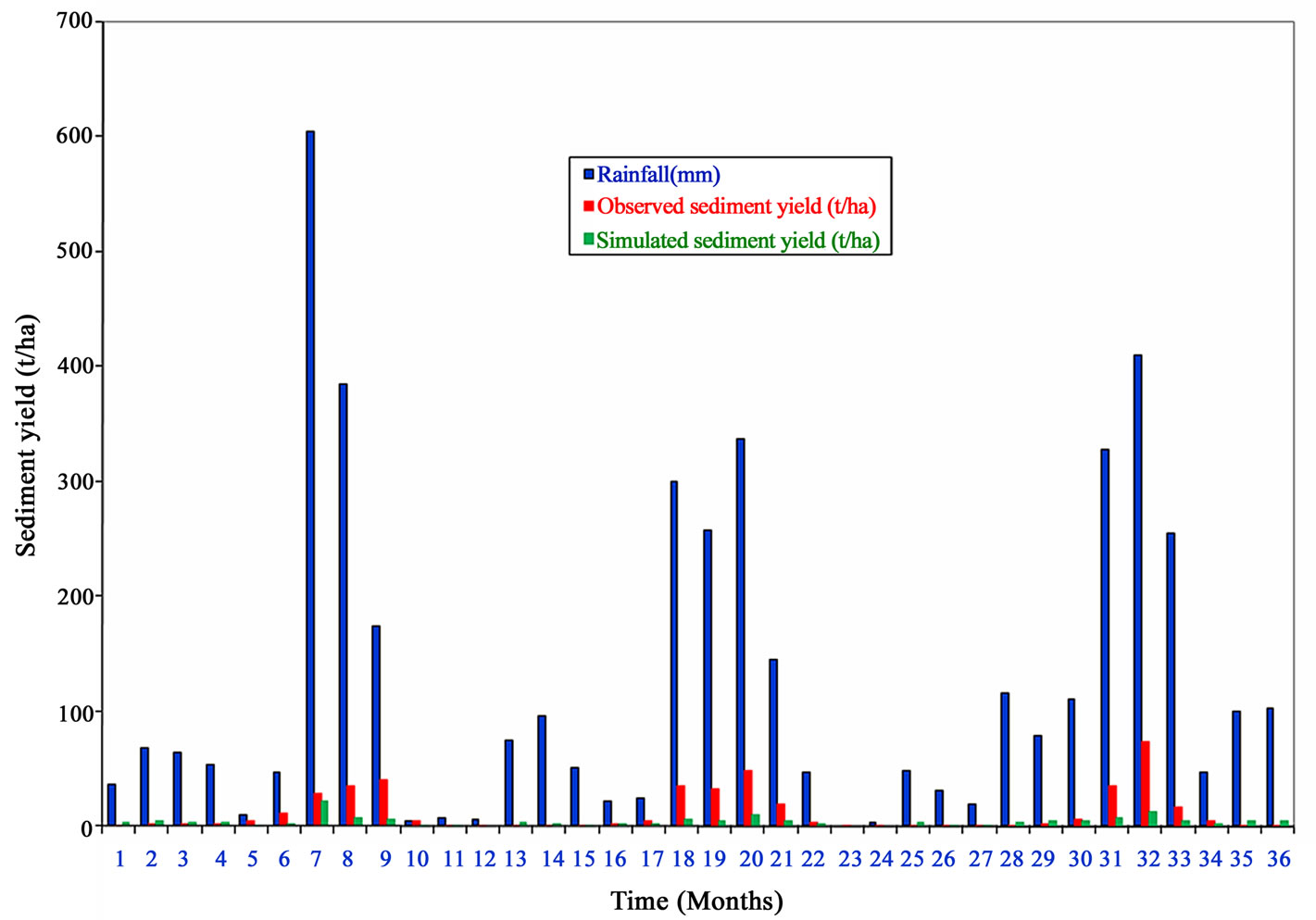 (b)
(b)
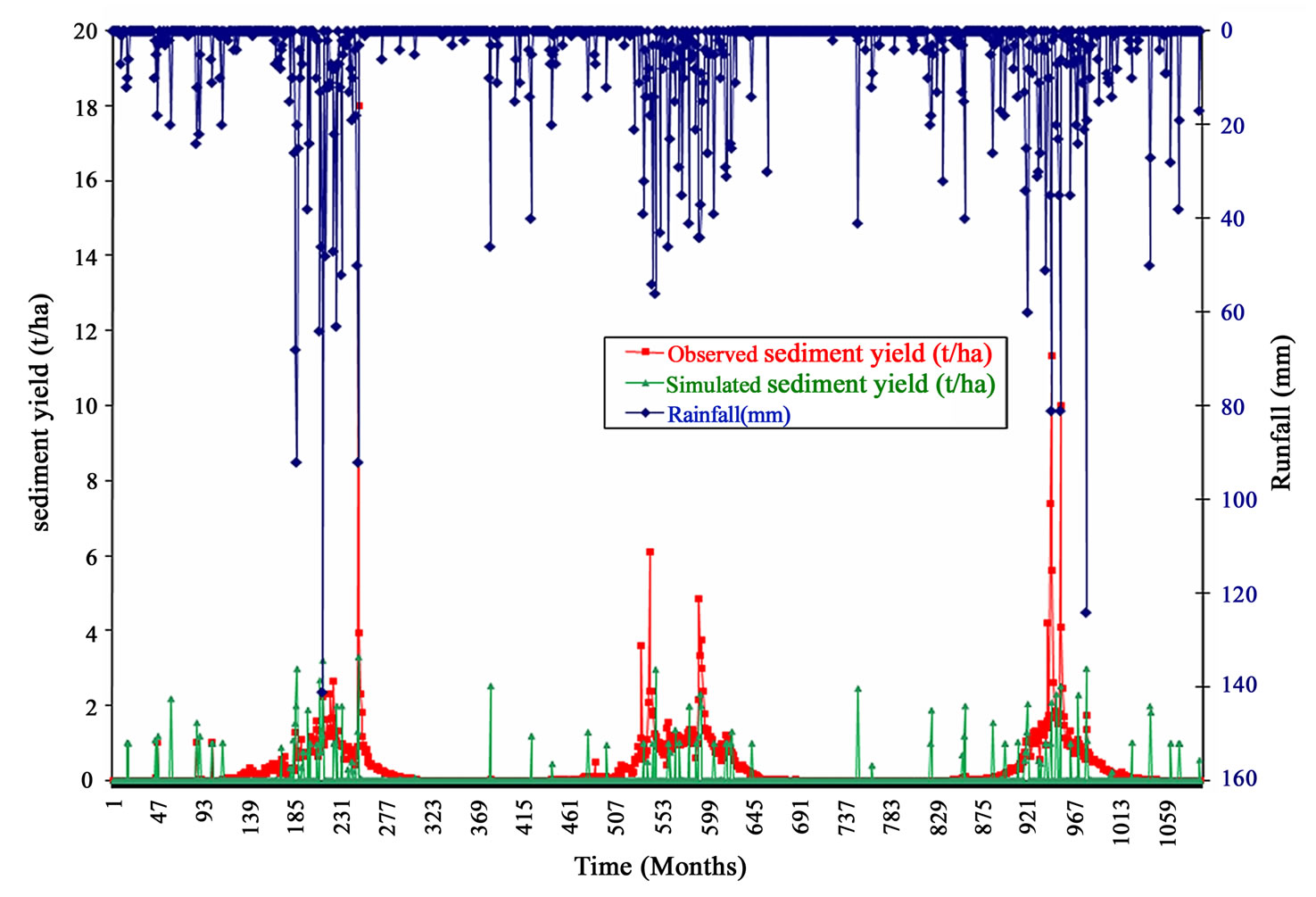
Figure 12. Comparison of observed and simulated. (a) daily sediment yield; (b) monthly sediment yield for the validation period 1995-97.
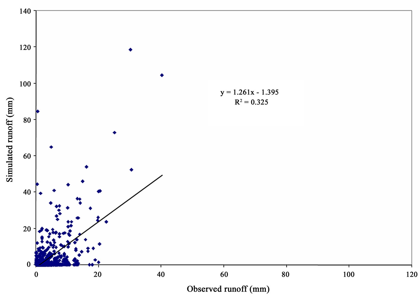
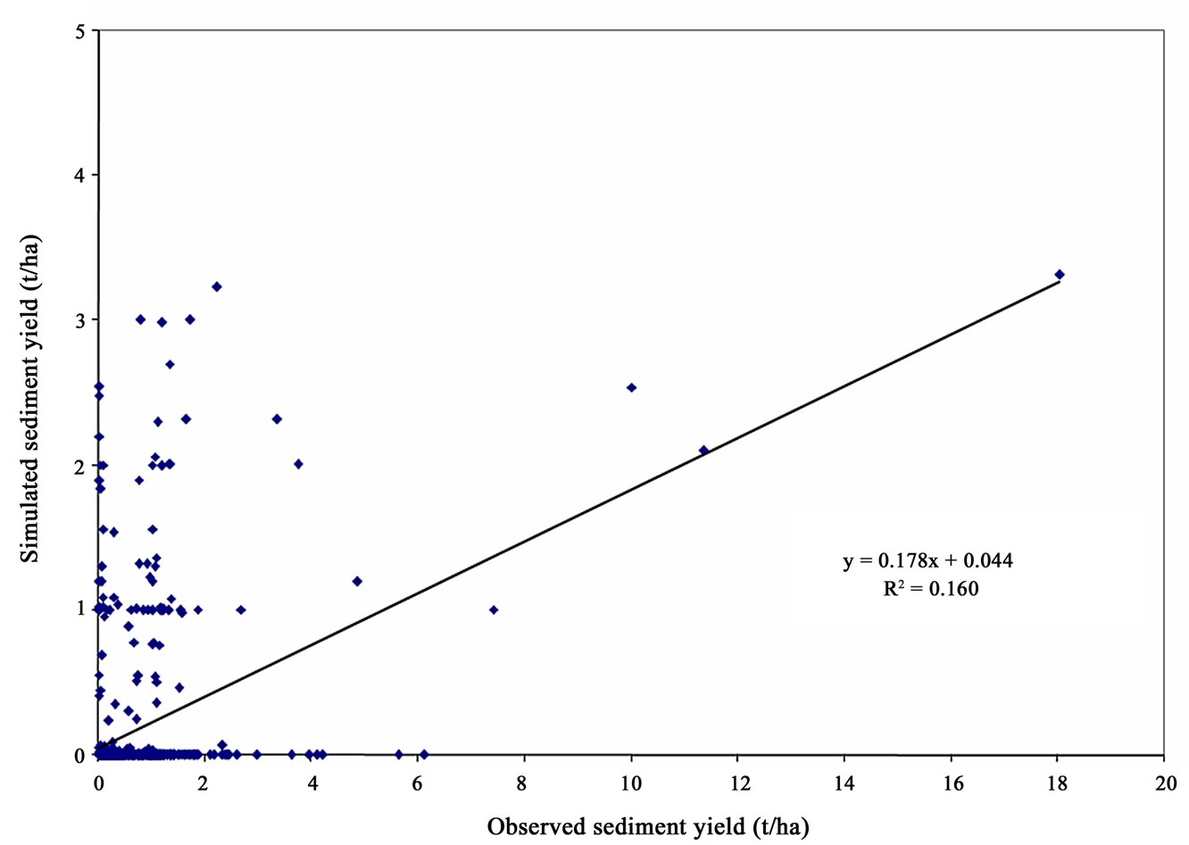
1996 and 1997, the simulated runoff was 957.13, 804.92 & 974.80 mm respectively as against the observed runoff of 931.47, 1252.68 and 1197.77 mm from a corresponding total rainfall of 1453, 1350 & 1641 mm. The plots of daily and monthly sediment yield (Figure 12(a), (b)) show that the sediment yield was underestimated by the model. The total sediment yield simulated by the model was computed to be 46.33, 31.13 & 44.36 t/ha as against the observed sediment yield of 125.21, 143.75 and 137.35 t/ha respectively for the years of 1995, 1996 and 1997. The R2 values for the daily and monthly runoff (Figure 13(a), (b)) were obtained as 0.33 and 0.62 respectively, while these values for sediment yield (Figure 14(a), (b)) were computed as 0.26 and 0.47 respectively for the validation period of 1995 to 1997.
The results of the study can further be assessed keeping in view the unreliability of the input data. The parameter values derived from various sources need to be
 (a)
(a)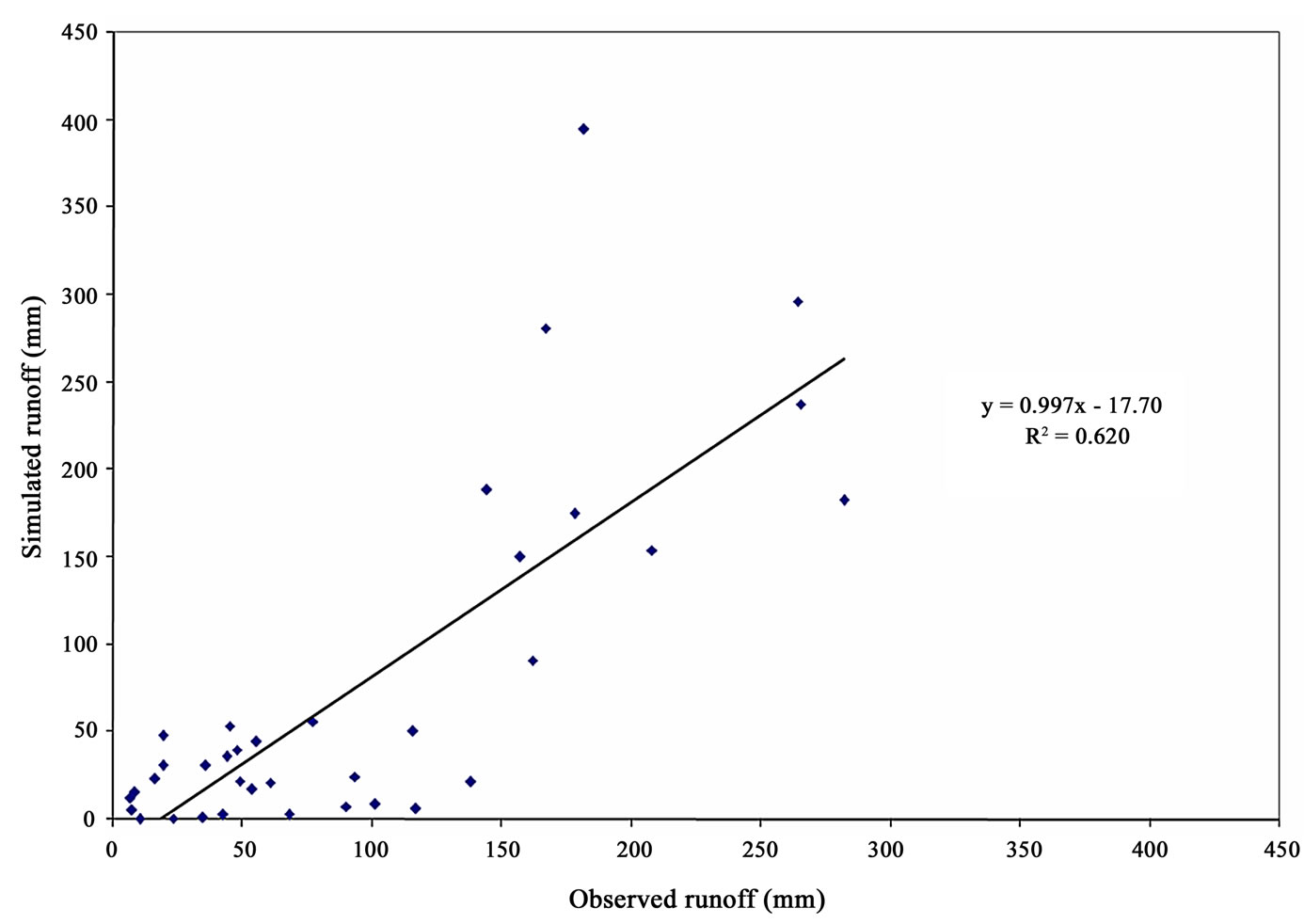 (b)
(b)
Figure 13. Goodness-of-fit for observed and simulated. (a) daily runoff; (b) monthly runoff for the validation period 1995-97.
 (a)
(a)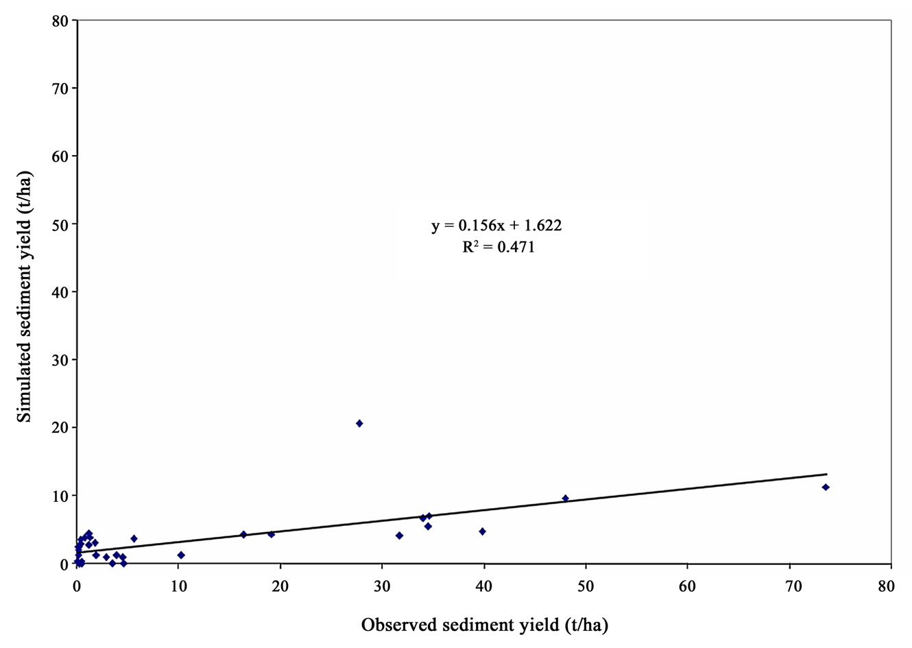 (b)
(b)
Figure 14. Goodness-of-fit for observed and simulated. (a) daily sediment yield; (b) monthly sediment yield for the validation period 1995-97.
verified in the field which is a difficult task in view of its approachability and mostly covered by thick forest. Similarly, the land use derived from remote sensing data was based on unsupervised classification. Further, the rainfall, runoff and sediment yield data used in the study may involve a number of possible human and instrumental errors. Keeping in view the above, it can be concluded from the simulation results of the study that the SWAT model has simulated the runoff and sediment yield reasonably well from an intermediate watershed in Himalayan region. The enhanced performance of the model could be achieved with some refinement in the input data.
5. Conclusions
In the present study, SWAT 2000, a physical based semi distributed hydrological model having an interface with ArcView GIS software was applied to a Himalayan watershed for modeling runoff and sediment yield. After preparing all the thematic maps and database as per the format of AVSWAT model, the model was calibrated for the daily and monthly surface runoff and sediment yield using the observed data of 1993 and 1994. The model validation was carried out for a data set of three years of 1995 through 1997. The simulation performance of the model for calibration and validation was evaluated using graphical and statistical methods.
The coefficient of determination (R2) for the daily and monthly runoff was obtained as 0.53 and 0.90 respectively for the calibration period and 0.33 and 0.62 respectively for the validation period. The R2 value in estimating the daily and monthly sediment yield during calibration was computed as 0.33 and 0.38 respectively. The R2 for daily and monthly sediment yield values for 1995 to 1997 was observed to be 0.26 and 0.47. The values of R2 can be considered reasonably satisfactory for estimating runoff and sediment yield from a remote watershed with scarce data.
REFERENCES
- J. G. Arnold, P. M. Allen, and D. Morgan, “Hydrologic model for design of constructed wetlands,” Wetlands, Vol. 21, No. 2, pp. 167–178, 2001.
- J. G. Arnold, and N. Fohrer, “SWAT2000: Current capabilities and research opportunities in applied watershed modeling,” Hydrology Process, Vol. 19, pp. 563–572, 2005.
- J. G. Arnold, R. S. Srinivasan, and J. R. Williams, “Large area hydrologic modeling and assessment: Part 1. Model development,” Journal of the American Water Resources Association, Vol. 34, No. 7389, 1998.
- J. Benaman, C. A. Shoemaker, and D. A. Haith, “Modeling non-point source pollution using a distributed watershed model for the Cannonsville Reservoir Basin,” Delaware County, New York. Proceedings of the World Water & Environmental Resources Congress, May 20-24, 2001.
- D. K. Borah and M. Bera, “SWAT model background and application reviews,” Paper Number: 032054, Presented at the ASAE Annual International Meeting, July 27-July 30, 2003, Las Vegas, Nevada, USA.
- K. Eckhartd and J. G. Arnold, “Automatic calibration of a distributed catchment model,” Journal of Hydrology, Vol. 251, pp. 103–109, 2001.
- N. Fohrer, D. Moller, and N. Steiner, “An interdisciplinary modeling approach to evaluate the effects of land
- use change,” Physics and Chemistry of the Earth, Vol. 27, pp. 655–662, 2002.
- A. Francos, G. Bidoglio, L. Galbiati, F. Bouraoui, F. J. Elorza, S. Rekolainen, K. Manni, and K. Granlund, “Hydrological and water quality modelling in medium sized coastal basin,” Physics Chemistry Earth (B), Vol. 26, No. 1, pp. 47–52, 2001.
- N. S. Hsu, J. -T. Kuo, and W. S. Chu, “Proposed daily streamflow-forecasting model for reservoir operation,” Journal of Water Resource Planning and Management, ASCE, Vol. 121, No. 2, 1995.
- M. Jha, W. Philip Gassman, S. Secchi, R. Gu, and J. Arnold, “Effect of watershed subdivision on SWAT flow, sediment and nutrient predictions,” Journal of American Water Resources Association, Vol. 40, No. 3, pp. 811– 825, 2004.
- K. W. King, J. G. Arnold, and R. L. Bingner, “Comparison of Green-Ampt and curve number methods on Goodwin Creek watershed using SWAT,” Transactions of the ASAE, Vol. 42, No. 4, pp. 919–925, 1999.
- J. E. Nash and J. V. Sutcliffe, “River flow forecasting through conceptual models Part I-a discussion of principles,” Journal of Hydrology, Vol. 10, pp. 282–290, 1970.
- S. L. Neitsch, J. G. Arnold, J. R. Kiniry, J. R. Williams, and K. W. King, “Soil and water assessment tool thereotical documentation - version 2000,” Soil and Water Research Laboratory, Agricultural Research Service, Grassland, 808 East Blackland Road, Temple, Texas.
- S. L. Neitsch, J. G. Arnold, J. R. Kiniry, R. Srinivasan, and J. R. Williams, “Soil and water assessment tool user’s manual - version 2000,” Soil and Water Research Laboratory, Agricultural Research Service, Grassland, 808 East Blackland Road, Temple, Texas.
- J. R. Peterson and J. M. Hamlett, “Hydrologic calibration of the SWAT model in a watershed containing fragipan soils,” Journal of the American Water Resources Association, Vol. 37, No. 2, pp. 295–303, 1998.
- J. Singh, K. H. Verman, and M. Demissie, “Hydrologic modelling of the iroquois river watershed using HSPF and SWAT,” Illinous State Water Survey Contract Report, 2004–2008, 2008.
- C. A. Spruill, S. R. Workman, and J. L. Taraba, “Simulation of daily and monthly stream discharge from small watersheds using the SWAT model,” Transactions of ASAE, Vol. 43, No. 6, pp. 1431–1439, 2000.
- M. P. Tripathi, R. K. Panda, and N. S. Raghuwanshi, “Identification and prioritisation of critical sub-watersheds for soil conservation management using SWAT model,” Biosystems Engineering, Vol. 85, No. 3, pp. 365 –379, 2003.
- E. Varanou, E. Gkouvatsou, E. Baltas, and M. Mimikou, “Quantity and quality integrated catchment modeling under climate change with use of soil and water assessment tool model” Journal of Hydrologic Engineering, Vol. 7, No. 3, pp. 228–244, 2002.