Advances in Chemical Engineering and Science
Vol.3 No.4(2013), Article ID:38785,10 pages DOI:10.4236/aces.2013.34037
Modeling a General Equation for Pool Boiling Heat Transfer
1Chemical Engineering Department, Higher Colleges of Technology, Abu Dhabi, United Arab Emirates
2Department of Chemical Engineering, Kuwait University, Kuwait City, Kuwait
3Mechanical Engineering Department, University of Technology, Baghdad, Iraq
Email: *mhameed@hct.ac.ae
Copyright © 2013 Mohammed Salah Hameed et al. This is an open access article distributed under the Creative Commons Attribution License, which permits unrestricted use, distribution, and reproduction in any medium, provided the original work is properly cited.
Received July 26, 2013; revised August 26, 2013; accepted September 5, 2013
Keywords: Pool Boiling; Nucleate Boiling; Linear and Non-Linear Technique Methods; Heat Transfer
ABSTRACT
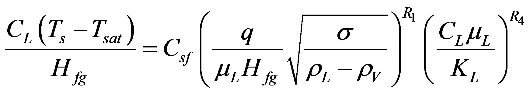
It is recognized that the nucleate pool boiling data available in literature are mainly related to four known correlations, each differs from the other by a varying magnitude of constant coefficients, depending on restrictive experimental conditions. The present work is concerned in developing an empirically generalized correlation, which covers the entire range of nucleate boiling with a minimum possible deviation from experimental data. The least squares multiple regression technique is used to evaluate the best coefficient value used in the correlations. An empirical correlation that fits a broader scope of available data has been developed by a non-linear solution technique leading to the following equation:  where the coefficients R1 and R3 both represent the effect of surface-liquid combination. They are assessed independently for the used surface material and liquid.
1. Introduction
Boiling is a complex process and an intensive work is needed for its understanding. Within the last decades, several nucleate boiling models were formulated and could be grouped in two main categories: a) Bubble Agitation Models and b) Macro/Micro Layer Evaporation Models.
The bubble agitation models are based on the principle of agitating the liquid, but they carry away little heat. The heat transfer is considered within the turbulent forced convection. The obtained empirical pool boiling heat transfer models employ dimensionless groups based on both fluid and solid properties while the main constant in the model is found to depend on the geometry of the heater. The models found in literature are useful within the range of database used in developing their derivation.
Bubble agitation mechanism together with Helmholtz-instability mechanism can be used either to explain the heat transfer at the low heat flux regime or to explain CHF (Critical Heat Flux). They cannot account for the continuity of the pool-boiling curve. On the other hand, the macro/micro layer evaporation reproduces the poolboiling curve from the nuclear boiling to transition boiling. The macro/micro layer models play an important role in high heat flux region. The liquid layer includes the micro layer underneath the bubble and the macro layer on the base of coalescence and dries out periodically [1]. Heramura & Katto [1] assume the liquid-vapor interface is stationary and the entire surface heat flux contributes to macro layer evaporation.
Several numerical models were proposed based on the macro layer theory among that of Maruyama et al. [2]. Zhao et al. [3] put forward a model for transient pool boiling heat transfer. The model employed is too high heating rate to be realized in practical experiments for a horizontal surface. He et al. [4] concluded that the macro layer model is more suitable for the high heat flux regime. Dhir [5] confirmed that numerical simulations are not a substitute for detailed experiments. The experimental results are needed to validate the simulations. Numerical simulations provide additional insights into the boiling phenomena.
Within the late decade, many researchers worked on viewing the pool boiling in microgravity (in the absent of buoyancy) to understand the lower limit of forced convection. Several workers are Lee [6], Herman [7], Wan & Zhao [8], and Kubota et al. [9].
Ji et al. [10] enhanced the pool boiling heat transfer in microgravity by using porous coating heating surface at atmospheric pressure and slightly moderate superheats.
Other researchers [11,12] enhanced the pool boiling by using nanofluid (water mixed with extremely small amount of nanosized particles). They concluded the enhancement of the thermal conductivity and convection heat transfer capability of the suspended particles of nanometer in size for many volume fractions of nanofluids.
The results of workers [6-12] can be used as a guidance in formulating proper equations that can be used in design. The aim of the present work is to use bubble agitation models to obtain a generalized empirical correlation that gives the best possible representation of collected data. Pool of data is collected from literature for various liquids effects with different plain test surfaces. For this purpose, linear and non-linear programming techniques were used in the evaluation of the proposed correlation.
2. Theoretical Analysis of Bubble Agitation Models
The primary requirement for nucleation to occur or for a nucleus to subsist in a liquid is that the liquid should be superheated. There are two types of nuclei. One type is formed in a pure liquid; it can be either a high energy molecular group resulting from thermal fluctuations of liquid molecules, or a cavity resulting from a local pressure reduction such as that occurs in accelerated flow. The other type, formed on a foreign object can be either a cavity on the heating wall or suspended foreign material with a non-wetted surface.
Rohsenow [13] assumes that the movement of bubbles at the instant of breaking away from the heating surface is of prime importance and obtained Equation (1) for heat transfer in the region of nucleation pool boiling.
 (1)
(1)
The recommended variation of r is within 0.8 to 2.0. Evaluation of Csf from experimental results of many workers [14] prove to be a parameter which does not pick out only the nucleation ability of heating surface but contains the effect of physical properties of liquid.
Rohsenow [15] proposed the surface factor Csf to prescribe the condition of heating surface in nucleate boiling. Various investigators [14] utilized this factor in their determination of empirical expressions. The surface factor is defined by Equation (1), generally known as Rohsenow empirical correlation.
Forster and Zuber [16] indicated that small bubbles grow rapidly and large ones slowly, but the degree of agitation in the surrounding liquid due to bubble growth remains the same. They derived the following empirical correlation:
 (2)
(2)
Equation (2) predicts the same heat transfer coefficient for a liquid boiling on any hot surface (for all heterogeneous cases only) or boiling in bulk (for all homogeneous cases only). Rohsenow’s Equation (1) was developed and applied to the heterogeneous case only.
Forster and Greif [17] suggested a different approach by considering that the mechanism of high heat transfer rate, during nucleate boiling, is mainly due to the liquidvapor exchange. They obtained a dimensional empirical correlation, for the pool boiling heat flux q in water at 100 - 4763 kN/m2, as shown in Equation (3).
 (3)
(3)
This correlation is not as widely verified as that of Rohsenow.
Gupta and Varshney [18] obtained experimental data for boiling heat transfer, using distilled water, benzene and toluene as liquids over a heated horizontal cylinder made of stainless steel. Their data was correlated by the following dimensionless empirical correlation:
 (4)
(4)
where NuB and PeB are the Nusselt and Peclet number of boiling respectively. Or it can be written as:
 (5)
(5)
In order to derive a general correlation based on bubble agitation phenomena to be more versatile than the correlations existing in literature, a search was made through published work in literature and found that the following four well known empirical correlations referred to in most publications:
a) Rohsenow correlation (Equation(1))
b) Forster and Zuber correlation (Equation (2))
c) Forster and Greif correlation (Equation (3))
d) Gupta and Varshney correlation (Equation (5)).
For the sake of analysis, experimental data collected from many literatures [19-24] tabulated as heat flux (q), surface temperature (Ts), heat transfer coefficient (h), and coefficient h* (equal to h/q0.7). Moreover, physical and thermodynamic properties collected at the reported experimental conditions from literature [25-29] to be used in the analysis. The properties include, liquid thermal conductivity (KL), liquid heat capacity (CL), density of vapor (rV), surface tension of liquid (s), saturation temperature (Tsat), density of liquid (rL), latent heat of vaporization (Hfg), and viscosity of liquid (mL).
The above stated correlations are of dimensionless form with the exception of the Forster and Greif correlation (Equation (4)). These equations can be represented by general equation as shown in Appendix. Many modifications to linear correlations have been tried to minimize the sum of squares of errors and to conclude some general correlations.
3. Results and Discussion
Boiling heat transfer studied earlier indicated that several variables are important in nucleate boiling such as pressure, fluid properties, surface condition, boiling temperature, kind and relative amount of impurities. The practical data showed that changes in magnitude of these properties and conditions could significantly affect pool boiling heat transfer.
A graphical analyses for 56 sets of literature data was used in studying the effect of heat flux, (q), and operating pressure (P), on boiling heat transfer coefficient, (h). Figures 1-3 show the variation of heat transfer coefficient with heat transfer flux, (q). The lines in the figures are the best-fit lines of the reported data. Figure 1 plotted for various liquids at different operating pressure and test surface. Figure 2 corresponds to various liquid-surface combinations at constant atmospheric pressure. Figure 3 reflects the behavior of various metal surfaces and operating pressures for the same liquid.
All the data can be represented by the empirical, Equation (6), with an average percentage error ranging from 0.012 to 11.8
 (6)
(6)
The proportionality constant h* is proved to be a function of pressure and liquid-surface combination. Cichelli
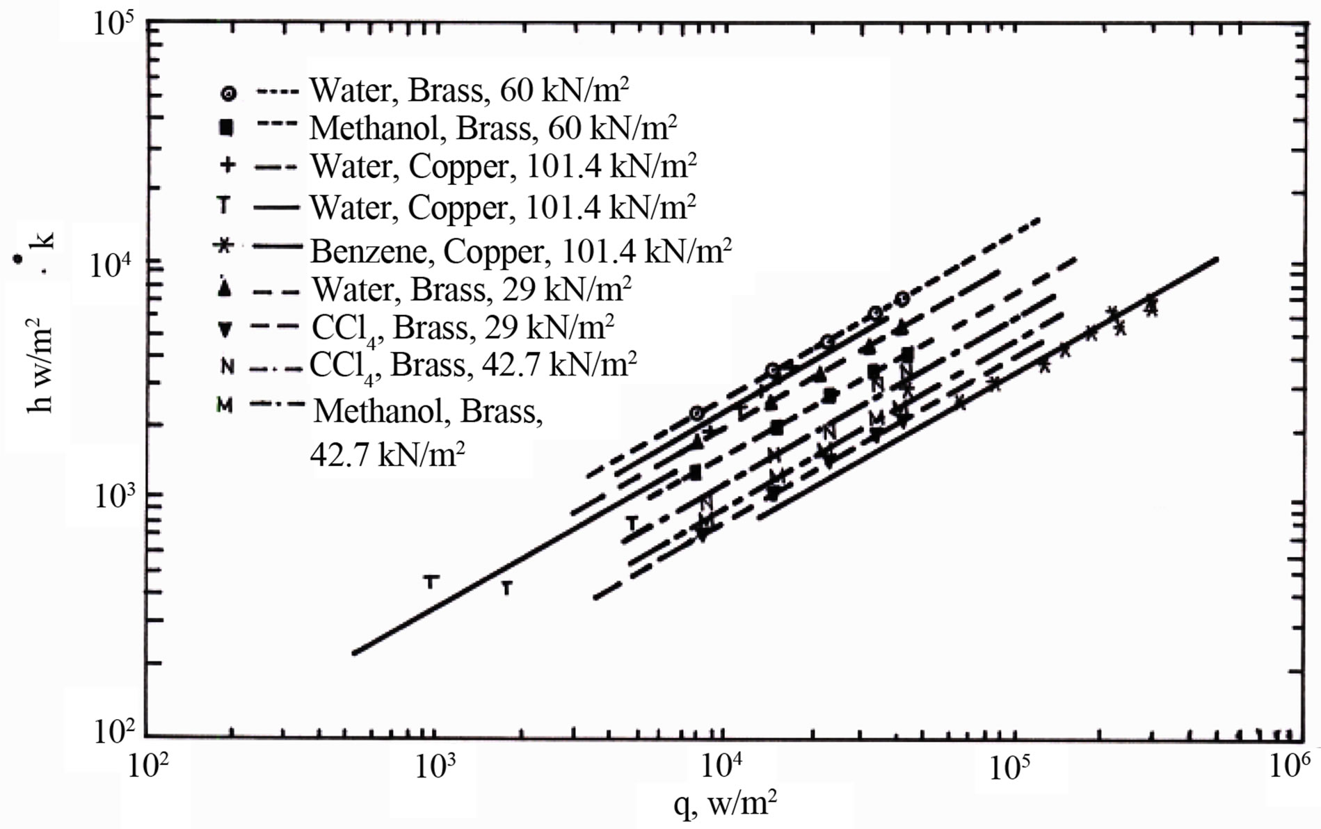
Figure 1. Heat transfer coefficient (h) versus heat flux (q) at various pressures.

Figure 2. Heat transfer coefficient (h) versus heat flux (q) at atmospheric pressure.

Figure 3. Heat transfer coefficient (h) versus heat flux (q) for various metal surfaces.
and Bonilla [19] confirmed that the coefficient of heat transfer increases with absolute operating pressure in the nucleate boiling zone. They reported the following correlation:
 (7)
(7)
Figure 4 shows the variation of the proportionality constant (h*) as function of pressure (P) for a definite liquid-surface combination. Equation (8) represents the relationship between h* and P, that was obtained from best data fit of Figure 4.
 (8)
(8)
The overall dependence of (h) on operating pressure (P) and heat flux (q) for different liquid-surface combinations is shown in Figure 5.
3.1. Linear Programming Analysis of Empirical Correlations
Equation (A.4) in Appendix used to test the validity of the published correlations. It is used to formulate a correlation that shows the best fit of the experimental data. All the data cited in the literature from [19-24] classified as eight liquids (Water, Benzene, Methanol, Carbon Tetrachloride, n-Butanol, Isopropanol, n-Amyl Alcohol, and n-Heptane) and four surfaces (Brass, Copper, Nichrome, and Stainless Steel) at different operating pressures grouped in 56 data sets.
The applicability of the four empirical correlations, Equations (1)-(3) and (5), in representing the data was test by using linear-programming; that by fixing some of
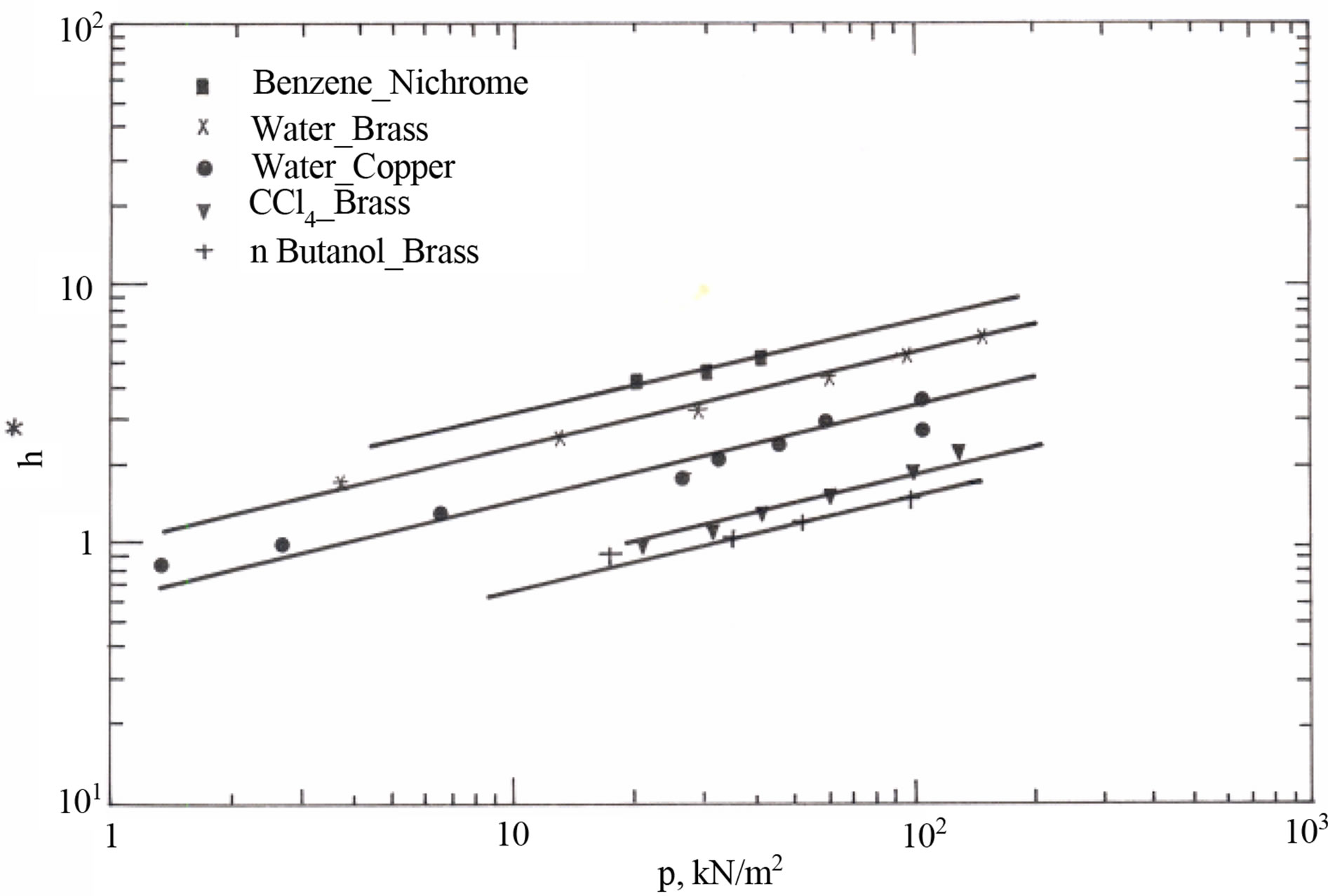
Figure 4. Proportionality constant (h*) versus operating pressure (P).
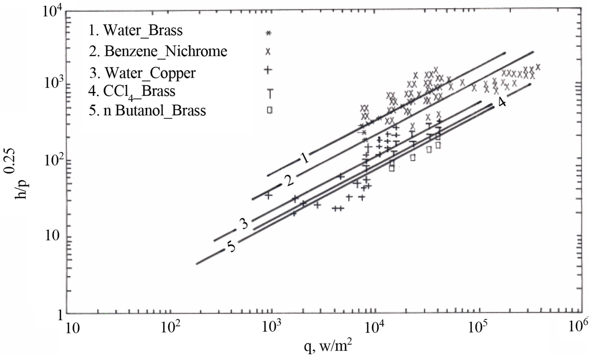
Figure 5. Heat transfer coefficient (h) dependence on operating pressure and heat flux (q).
the coefficients and evaluating the others and the average percentage error is used as test criteria for comparison purposes.
3.1.1. Rohsenow’s Correlation
Equation (9) is a general expression for Rohsenow’s correlation while the exact expression stated as in Equation (1).
 (9)
(9)
The coefficient Csf reported, in the literature, to vary with each liquid-surface combination and it is independent of pressure [22]. The validity of Equation (9) was tested for the entire collected data by applying the leastsquares method.
In the initial analysis of data, the pressure was assumed constant and the obtained results showed inconsistency in the calculated values of constants for various experimental conditions tested. The inconsistency in values of constants is most likely due to pressure effect, which was not considered as variable during the initial analysis of data. On the next try, a pressure parameter was introduced in an attempt to narrow the variation in the values of constants for different systems and to conclude general correlation. Four different expressions of pressure parameter cited from literature [16], and stated in Equation (10), was used and expected to have an effect on heat transfer in the region of pool boiling nucleation:
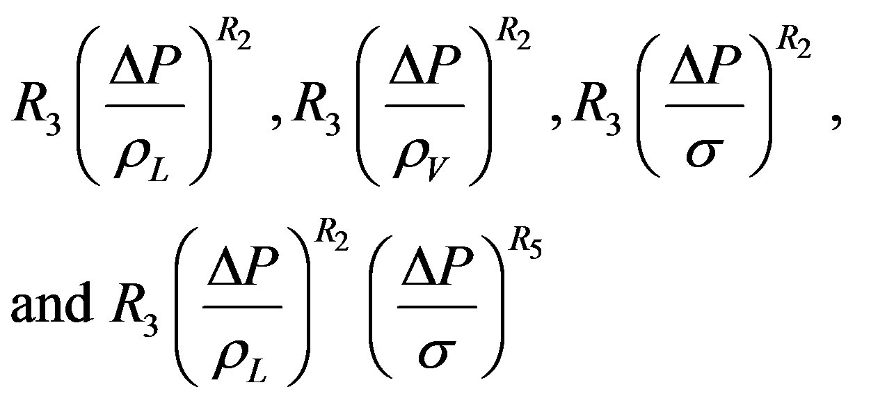 (10)
(10)
Each of these pressure expressions selected to replace the coefficient Csf in Equation (9) and the obtained results were compared and checked. The analysis found that the pressure parameter 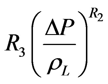 gives the lowest minimum percentage error between the others forms and selected to replace Csf and modify Equation (9) to the form showing in Equation (11).
 (11)
(11)
To make the present work more general, the analysis was repeated for various liquids at certain test surface and different operating pressures, that by calculating all the coefficients (R1, R2, R3, and R4) of Equation (11) for each set of data. The values of coefficients were selected, by the help of Equation (A.4), on the basis of using Equation (11) with the lowest average percentage error.
3.1.2. Gupta and Varshney Correlation
Equation (12) is a general expression for Gupta and Varshney empirical correlation, while Equation (5) represent the exact form.
 (12)
(12)
The pressure term is not included in the correlation of Gupta and Varshney as was the case of Rohsenow’s empirical correlation, Equation (1). Equation (12) differs from Rohensow’s Equation (9) by including the density ratio term and classifying other dimensionless term in well-known groups. A similar data analysis used for Equation (12) as it was with the case of Rohsenow’s Correlation. By substituting the various pressure forms of Equation (10) in place of coefficient R3 in Equation (12), it is found that pressure expression  gave the minimum average percentage error. This term is then chosen as the best fit expression for pressure and used in Equation (12) to obtain Equation (13).
 (13)
(13)
In order to make the present work more general, the analysis repeated for various liquids at specific test surface and different operating pressures then follow the same procedure as in case of Rohsenow’s correlation. The analysis concluded that the modified Equation (13) provides a better data fit than that of Gupta and Varshney Equation (5).
3.1.3. Forster and Zuber Correlation
Equation (14) is a general expression for Forster and Zuber empirical correlation, while the exact form is given in Equation (2).
 (14)
(14)
The pressure term is taken care of in Forster and Zubers correlation, Equation (2). By applying a similar procedure as in previous cases, it was found that the validity of the above equation is restricted to specific experimental data near critical temperature difference. By checking the above results for Forster and Zuber empirical correlation, Equation (14), it is found that the overall average percentage errors is very high in predicting the published data under consideration.
3.1.4. Forster and Greif Empirical Correlation
Equation (15) is a general expression for Forster and Greif dimensional empirical correlation, while the exact form is given in Equation (3).
 (15)
(15)
Using the same sets of data analyzed previously gave a higher average percentage error as compared with the dimensionless empirical correlations as shown in Table 1.
The variation of some thermodynamic properties as function of pressure and temperature is not reported in literature and these properties were considered constant during the calculations, which may be the cause of the large average percentage error. Moreover, this empirical correlation dealt with fluid side effect of the problem and ignored the surface side effect on the nucleate boiling behavior. This might have added more error to the validity of this correlation.
The linear programming analysis recommended the use of the modified correlations of Rohsenow and Gupta & Varshney as they give closer prediction to the experimental data than in case of using Forster & Zuber and Forster & Greif modified correlations as showing in Table 1. Hence, the last two correlations excluded from any further analysis.
Table 1. Linear programming results for Equation (11) to Equation (15).
Where APE = Average Percentage Errors; CC = Correlation Coefficient.
3.2. Non-Linear Programming Analysis of Empirical Correlations
The data were re-analyzed by non-linear programming methods by using the modified correlations of Rohsenow, Equation (11), and Gupta & Varshney Equation (13) in an attempt to improve the correlations for lower average percentage error.
By assume that: 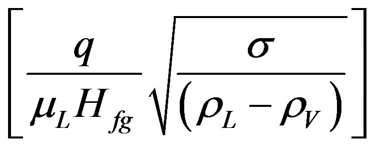 in Equation (4) is equal to X and
 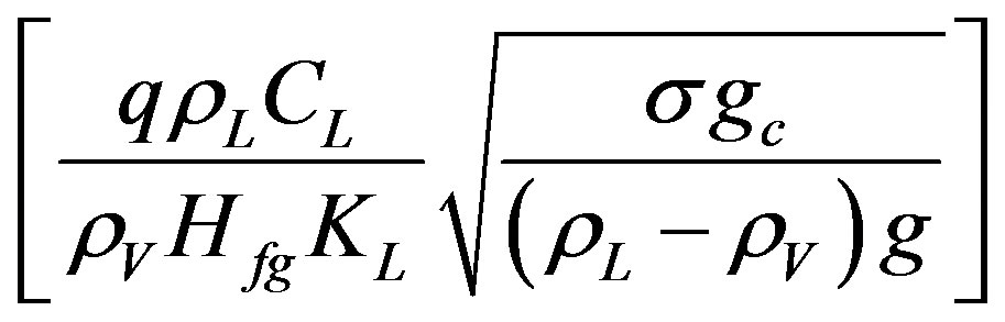 in Equation (13) is equal to Y, then use either of the following equations:
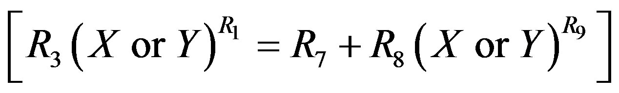
Binominal Expression:
 (16)
(16)
or non-linear Expression:
 (17)
(17)
to replace the  in Equation (11) or
  in Equation (13) respectively. It is found from data fittings that a better representation can be obtained by using the binominal expression, Equation (16), with
  in place of
  in Equation (11) and using the binominal expression, Equation (16), with
  in place of
  in Equation (13).
Various forms of expressions for the constant R7 was tried for both Rohsenow and Gupta & Varshney modified correlations. It was found that keeping R7 as a constant and independent of other parameters yielded a better data representation. It was also concluded that the average percentage error would not be improved by using the non linear equations instead of the linear equation as showing in Table 2.
General Empirical Correlation
By using the best data fit for Equation (11) for different surfaces (Nichrome, Copper, Brass, and Stainless Steel), the variation of the powers of pressure expression term and Prandtl number in the equation were found to be approximately equal to 0.08 and 1.0 respectively leading to the following generalized Equation (18).
 (18)
(18)
The coefficients R1 and R3 represent the effect of surface-liquid combination. They are assessed independently for each surface by the least-squares linear regression method and the results are stated in Table 3.
A similar analysis tried for Equation (13) and concluded that the powers of pressure term, Peclet number (PeB), and density ratio term (rV/rL) were relatively independent of surface—liquid combination as compared with the coefficient R3 and the power of Prandtl number, R4. The best form of Equation (13) was tested for different data sets and concluded Equation (19).
 (19)
(19)
A similar way was followed for Equation (19), to that of Equation (18), in finding the power R4 and the coefficient R3 and their best values are given in Table 3. The result of analysis of Equation (18) and Equation (19) listed in Table 3 suggested the use of Equation (19) in preference to Equation (18).
The applicability of Equaiton (19) was examined for different surfaces as showing in Figures 6-9. The equation found to fit well for all the data with the exception of Brass. The deviation in the results for Brass is due to

Table 2. Comparison of linear, binominal, and non linear expressions versions of Equations (11) and (13).

Table 3. Linear programming results for Equations (18) and (19).

Figure 6. Experimental data predictions using Equation (19) for Nichrome surface.

Figure 7. Experimental data predictions using Equation (19) for Copper surface.

Figure 8. Experimental data predictions using Equation (19) for Brass surface.
Figure 9. Experimental data prediction using Equation (19) for Stainless Steel surface.
limited available data at very low pressure. Equation (20) represents the dimensionless form of Equation (19).
 (20)
(20)
The analysis concluded that Equation (20) is valid for the entire available data and represent a more generalized correlation than the correlations found in literature.
4. Conclusions
A graphical analysis concluded that the empirical Equation (6) is showing the effect of heat flux (q) and operating pressure (P) on the boiling heat transfer coefficient (h).
 (6)
(6)
where h* is a function of pressure and for different liquid-surface combinations, it is found to vary with the pressure as follows:
 (8)
(8)
56 sets of literature data were tested on each of the four known correlations, Rohsenow, Forster & Zuber, Forster & Greif, and Gupta & Varshney, by using the linear and non-linear programming solution. The concluded results show that any of these correlations does not fit the entire data satisfactory. To improve their predictions, the correlations were modified, including additional parameters in an attempt to close up the deviation in the values of calculated parameters. The modified correlations of Rohsenow and Gupta & Varshney responded better to the applied modification than that of Foster & Zuber and Foster & Grief and they were considered for further analysis.
The least squares multiple regression technique [30,31] is used to evaluate the best possible values of the constant coefficients in the correlation. The cumulative error squares were minimized by using an ordinary optimum seeking technique. Linear, binominal & non-linear correlations were tested in concluding the final correlation.
The use of non-linear solution technique did not improve correlations 11 and 13 that were concluded by the linear technique and hence Equation (20) gives the best representation of the entire tested data.
REFERENCES
- Y. Haramura and Y. Katto, “A New Hydrodynamic Model of Critical Heat Flux, Applicable Widely to Both Pool and Forced Convection Boiling on Submerged Bodies in Saturated Liquids,” International Journal of Heat and Mass Transfer, Vol. 26, No. 2, 1983, pp. 389-399. http://dx.doi.org/10.1016/0017-9310(83)90043-1
- S. Maruyama, M. Shoji and S. Shimizu, “A Numerical Simulation of Transition Boiling, Heat Transfer,” Proceedings of the 2nd JSME-KSME Thermal Engineering Conference, Kitakyushu, 19-21 October 1992, pp. 345- 348.
- Y. H. Zhao, T. Masuoka and T. Tsuruta, “Theoretical Studies on Transient Pool Boiling Based on Microlayer Model (Mechanism of Transition from Nonboiling Regime to Film Boiling),” Trans. JSME (B), Vol. 63, No. 607, 1997, pp. 218-223.
- Y. He’ M. Shoji and S. Maruyama; “Numerical Study of High Heat Flux Pool Boiling Heat Transfer,” International Journal of Heat and Mass Transfer, Vol. 44, No. 12, 2001, pp. 2357-2373. http://dx.doi.org/10.1016/S0017-9310(00)00269-6
- V. K. Dhir; “Numerical Simulation of Pool-Boiling Heat Transfer,” AICHEJ, Vol. 47, No. 4, 2001, p. 813. http://dx.doi.org/10.1002/aic.690470407
- H. S. Lee, “Mechanisms of Steady-State Nucleate Pool Boiling in Microgravity,” Annals of the New York Academy of Sciences, Vol. 974, 2002, pp. 447-462. http://dx.doi.org/10.1111/j.1749-6632.2002.tb05924.x
- H. Herman, “Some Parameter Boundaries Governing Microgravity Pool Boling Modes,” Annals of the New York Academy of Science, Vol. 644, 2006, pp. 629-649.
- S. X. Wan and J. Zhao, “Pool Boiling in Microgravity: Recent Results and Perspectives for the Project DEPASJ10,” Microgravity Science and Technology, Vol. 20, No. 3-4, 2008, pp. 219-224.
- C. Kubota, et al., “Experiment on nucleate Pool Boiling in Microgravity by using Transparent Heating Surface- Analysis of Surface Heat Transfer Coefficients,” Journal of Physics: Conference Series, Vol. 327, 2011, Article ID: 012040.
- X. Ji, J. Xu, Z. Zhao and W. Yang, “Pool Boiling Heat Transfer on Uniform and Non-uniform Porous Coating Surfaces,” Experimental Thermal and Fluid Science, Vol. 48, 2013, pp. 198-212. http://dx.doi.org/10.1111/j.1749-6632.2002.tb05924.x
- S. H. You, J. H. Kim and K. H. Kim, “Effect of Nano Particle on Critical Heat Flux of Water in Pool Boiling Heat Transfer,” Applied Physics Letters, Vol. 83, No. 16, 2003, pp. 3374-3376. http://dx.doi.org/10.1063/1.1619206
- S.K. Das, N. Putra and W. Roetzel, “Pool Boiling Characteristics of Nano-Fluid,” International Journal of Heat and Mass Transfer, Vol. 46, No. 5, 2003, pp. 851-862. http://dx.doi.org/10.1016/S0017-9310(02)00348-4
- W. M. Rohsenow and J. A. Clark, “Heat Transfer and Fluid Mechanics,” Inst. Stanford University Press, 1951, p. 193.
- K. Nishikawa and Y. Fujita, Memoirs of the Faculty of Engineering, Kyushu University, Vol. 36, No. 2, 1976, p. 136.
- W. M. Rohsenow, Trans. ASME, Vol. 74, 1952, p. 966.
- H. K. Forster and N. Zuber, “Dynamics of Vapor Bubbles and Boiling Heat Transfer,” AIChE Journal, Vol. 1, No. 4, 1955, p. 531. http://dx.doi.org/10.1002/aic.690010425
- H. K. Forster and R. A. Grief, Journal of Heat Transfer, Vol. 81, No. 1, 1959.
- S. C. Gupta and B. S. Varshney, International Journal of Heat and Mass Transfer, Vol. 23, 1980, p. 219.
- M. T. Cichelli and C. F. Bonilla, Trans. AICHE, Vol. 41, 1945, p. 755.
- D. S. Cryder and A. C. Finalborgo, Trans. AICHE, Vol. 33, 1937, p. 346.
- C. V. Sternling and L. J. Tichacek, “Heat Transfer Coefficients for Boiling Mixtures: Experimental Data for Binary Mixtures of Large Relative Volatility,” Chemical Engineering Science, Vol. 16, No. 3-4, 1961, pp. 297-337. http://dx.doi.org/10.1016/0009-2509(61)80040-7
- I. A. Rabin, R. T. Beaubuef and G. E. Commerford, Chemical Engineering Progress Symposium Series, Vol. 61, No. 57, 1965, p. 249.
- G. S. Yadav and O. P. Chawla, Mechanical Engineering Division, Vol. 60, Part ME. 6, 1980, p. 229.
- A. A. Mahdi, “Pool Boiling of Saturated Liquids,” M.Sc. Thesis, University of Technology, Baghdad, 1983.
- E. A. Farber and E. L. Scorah, Trans. ASME, Vol. 70, 1948, p. 369.
- ESDU Engineering Sciences Data Unit, Chemical Engineering Series, Physical Data, Vol. 2, 1978.
- ESDU Engineering Science Data Unit, Chemical Data, Vol. 4, 1978.
- E. W. Washburn, “International Critical tables of Numerical Data, Physics, Chemistry and Technology,” McGraw-Hill Book Company Inc., New York, 1926.
- R. H. Perry and C. H. Chilton, “Chemical Engineers Handbook,” 4th Edition, McGraw-Hill Kogakusha, Ltd., 1963.
- C. Brice, H. A. Luther and O. W. James, “Applied Numerical Methods,” John Wiley and Sons, Inc., Hoboken, 1969, p. 272.
- P. R. Adby and M. A. H. Demoster, “Introduction to Optimisation Methods,” Chapman and Hall, 1974. http://dx.doi.org/10.1007/978-94-009-5705-3
Appendix
Sum of Squares of Errors
Equations (1) to (4) can be represented by a general equation:
where 
 (A.1)
(A.1)
This equation represents a general form of those correlations and simplified by taking logarithms of both sides.

or
 (A.2)
(A.2)
For N number of data readings there will be N number of linear equations, while for the determination of k coefficients only k equations are required. A least squares multiple regression technique [30,31] was used to evaluate the best possible coefficient from raw data readings. The cumulative error squares minimized by an ordinary optimum seeking technique [31] resulting into k number of equations to provide k number of coefficients for the entire data. These equations mathematically represented in the form:
 (A.3)
(A.3)
The sum of squares of errors is expressed as:
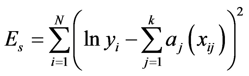 (A.4)
(A.4)
Nomenclature
CL—Heat capacity of liquid, J/kg×˚C Csf—Surface factor Fm—Nucleation factor g—Acceleration of gravity, m/s2
gc—Conversion ratio, kg m/kg·s2
h—Heat transfer coefficient W/m2·˚C h*—Proportionality constant Hfg—Latent heat of vaporation, J/kg KL—Thermal conductivity, W/m ˚C NuB—Nusselt number for boiling = 
P—Operating pressure (kN/m2)
PeB—Peolet number for boiling = 
Pr—Prandtl number q—Heat Flux, W/m2s
 —coefficients Re—Reynolds number Reb—Reynolds number for bubbles =
Sr—Superheat ratio = 
Ts—Test surface temperature, ˚C Tsat—Saturation temperature, ˚C
Greek Letters
aL Thermal diffusivity, m2/s, 
DP Pressure difference corresponds to (Ts–Tsat), kN/m2
mL Viscosity of liquid, kg/m×s rV Density of vapor, kg/m3
rL Density of liquid, kg/m3
s Surface tension, kg/s2
Subscripts
b Refers to bubble property
B Refers to boiling condition
L Refers to liquid condition
sf Refers to surface factor
s Refers to surface condition
sat Refers to saturation condition
v Refers to vapor condition
NOTES
*Corresponding author.