Natural Resources
Vol.4 No.1(2013), Article ID:29185,13 pages DOI:10.4236/nr.2013.41011
Sedimentation in Mountain Streams: A Review of Methods of Measurement
![]()
1Division of Forestry and Natural Resources, West Virginia University, Morgantown, USA; 2US Geological Survey, West Virginia Cooperative Fish and Wildlife Research Unit, West Virginia University, Morgantown, USA; 3Department of Civil and Environmental Engineering, West Virginia University, Morgantown, USA.
Email: larahedrick@frontiernet.net
Received November 19th, 2012; revised December 21st, 2012; accepted January 16th, 2013
Keywords: Mountain; Samplers; Sediment; Streams
ABSTRACT
The goal of this review paper is to provide a list of methods and devices used to measure sediment accumulation in wadeable streams dominated by cobble and gravel substrate. Quantitative measures of stream sedimentation are useful to monitor and study anthropogenic impacts on stream biota, and stream sedimentation is measurable with multiple sampling methods. Evaluation of sedimentation can be made by measuring the concentration of suspended sediment, or turbidity, and by determining the amount of deposited sediment, or sedimentation on the streambed. Measurements of deposited sediments are more time consuming and labor intensive than measurements of suspended sediments. Traditional techniques for characterizing sediment composition in streams include core sampling, the shovel method, visual estimation along transects, and sediment traps. This paper provides a comprehensive review of methodology, devices that can be used, and techniques for processing and analyzing samples collected to aid researchers in choosing study design and equipment.
1. Introduction
Over the past few decades, many studies have summarized sedimentation as the single greatest water pollutant affecting streams throughout the United States [1-3]. In the 1982 National Fisheries Survey, Reference [1] reported that respondents (fisheries managers with greater than 9 years experience in states throughout the US) ranked sedimentation as the major concern in all streams, and excessive sedimentation ranked number one in sources adversely affecting fishery habitats. Based on the US EPA 1992 inventory of stream and water quality, sedimentation affected 45% of impaired stream miles in the United States [4].
Sedimentation in streams can be defined in two ways, 1) the concentration of suspended sediment, or turbidity; and 2) deposited sediment, or sedimentation on the streambed [5]. Land uses that have the greatest potential to impact stream sediment include agriculture, forestry, mining, urban development, and the construction of pipelines and roads related to natural gas drilling [5-7]. The negative biological effects of sediment have been well documented in both experimental and observational studies [8,9]. Increased deposition of fine sediment can smother the streambed making it unsuitable as habitat for many plants and animals. Transported material can affect the biota directly through abrasion, and indirectly, by modifying the behavior of benthic fauna [10,11].
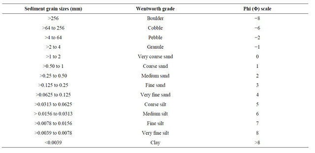
Particle size refers to the diameter of individual grains of sediment. Size ranges define limits of classes that are given names in the Wentworth scale [12]. Wentworth’s grades and sizes were later supplemented by William Krumbein’s phi or logarithmic scale, which transforms the millimeter number by taking the negative of its logarithm in base 2 to yield simple whole numbers (Table 1). The size fraction larger than sand (granules, pebbles, cobbles and boulders) is collectively called gravel, and the size fraction smaller than sand (silt and clay) is collectively called mud. Printed cards, called comparators, are used to determine grain sizes in the field. In the laboratory, standard sieves can be used [13].
Often fine sediment is determined by the grain size that negatively impacts the biological health of the stream. In mountain streams this is often related to salmonid egg and fry survival. Reference [14] classified fine sediment as <4 mm, as this size class is widely accepted as the critical one for western salmonids. References [15,16] reported a negative relation between brook trout (Salvelinus fontinalis) egg and fry survival when fine sediments comprised 20 - 25 percent of the bed substrate. Reference
Table 1. The Wentworth grain size scale and corresponding Phi scale values.
[17] showed that sediment between 0.063 mm and 1 mm diameter had a negative effect on spawning substrate quality and brook trout populations in West Virginia. Reference [18] defined fines as 0.74 - 8 mm in a study done on effects of fire and dam failure on the Boise National Forest. Reference [19] defined fines as <2.28 mm in diameter. Reference [20] classified three levels of fines <3.35, <1.75, and <0.85 mm in diameter.
Quantitative measures of stream sedimentation are useful to monitor and study anthropogenic impacts on stream biota, and stream sedimentation is measurable with multiple sampling methods. Evaluation of sedimenttation can be made by measuring the concentration of suspended sediment, or turbidity, and by determining the amount of deposited sediment, or sedimentation on the streambed [21]. Turbidity is a measure of the collective optical properties of a water sample that cause light to be scattered and absorbed [22,23]. Suspended sediment is usually the major contributor to turbidity; however, other materials are also contributors, such as plankton and organic detritus. Turbidity is typically measured in nephelometric turbidity units (NTU), and is done in the field using a nephelometer. Suspended sediments are typically measured in parts per million (ppm; mg/L), from grab samples filtered, dried, and weighed in the laboratory [22, 23].
Measurements of deposited sediments are more time consuming and labor intensive than measurements of suspended sediments. Traditional techniques for characterizing sediment composition in streams include core sampling [24-26], the shovel method [27,28], visual estimation along transects [25,29], and sediment traps [20,30, 31].
2. Materials and Methods
2.1. Core Sampling
The original McNeil Ahnell core sampler technique was published in 1964. Prior to the creation of this sampling device, “core sampling” was done using open cylinders [24]. The original sampler was designed to collect a standard volume of spawning gravel to a depth of 23 cm. The device has four basic parts: a coring cylinder, a collection cylinder, a coring handle, and a plunger cap (Figure 1). There is a stop ring inside the coring cylinder which provides a consistent marker for depth of the sample. It also acts as the platform for the plunger which seals the sample into the collection cylinder after excavation from the core sample area.
The technique involves sinking a stainless steel round sampler into the substrate by applying downward pressure and rotation. This is done until the sediment reaches the stop ring, then the contents of the coring cylinder are excavated by hand into the collection cylinder. It is important to scoop the material and then rinse hands in the collection basin. Once the coring cylinder has been excavated the plunger is fitted into the coring cylinder and the sample is transferred to a 19 liter bucket. A wash bottle is used to rinse all the fines into the bucket [32].
The McNeil Anhell sampler has been modified by various researchers to meet specific needs [20,25]. Other researchers have used different materials to construct a core sampling device. Reference [33] used a plexiglass tube to obtain a core sample. Reference [34] collected samples using a 125 liter drum. The subsurface material was removed to a depth of about one diameter of the largest surface grains.
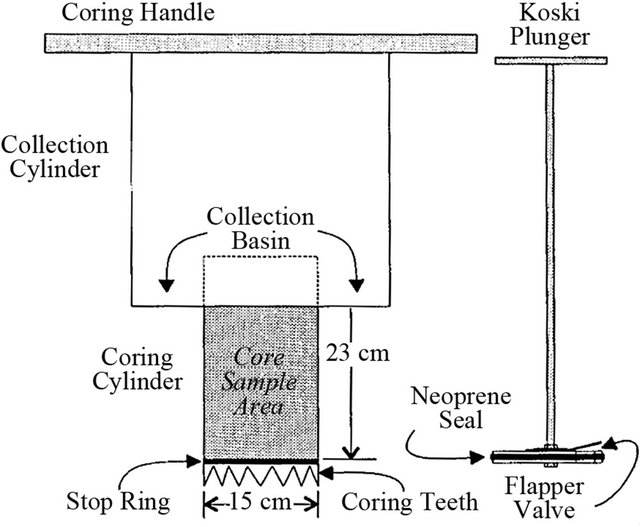
Figure 1. McNeil-Anhell core sampler.
Core sampling is effective, but can be labor and equipment intensive, and it is difficult to insert the sampler to a specified depth in coarse or compacted substrate [25]. The McNeil core sampler weighs about 11.3 kg. This can make it difficult to transport to remote locations. Samples are also heavy, weighing up to 18 kg and are often difficult to transport due to the large amount of water collected [28].
Once samples are collected they can by analyzed in the laboratory using the “dry” method or in the field using the “wet” method. Sediments and water collected are strained through a series of sieves or samples are dried in the lab and then sieved to determine the particle size distribution, or percent fines.
2.2. Shovel Method
The shovel method produces lighter samples, which are less costly, and can be taken more quickly than the McNeil sampler [27,28]. Shovel sampling entails pushing the blade into the desired location in the streambed to about half way up the length of the blade. The handle of the shovel then is pushed downward to lever the blade out of the bed. The shovel blade is slowly lifted from the stream, and water is allowed to drain from the sample before storing it in a zipper-lock plastic bag. During extraction and transference to the bag, care is taken to avoid losing the smallest fraction of the sample.
Shovel samples can vary in size and weight depending on the technique used. Reference [35] used a shovel to collect a 1 m2 area by excavating to the depth of penetration of the coarsest surface particle. Samples varied in weight from 27 - 35 g. Reference [28] designed three shovel-based methods: a standard number 2 round-point shovel (S1), a shovel with a portable stilling well (S2), and a modified shovel with side walls (S3). The standard number 2 round-point shovel (S1) was 23 cm long and 21 cm wide. Samples were collected facing upstream.
The second method was a standard number 2 round-point shovel with a portable stilling well (S2) fabricated out of four 64 cm sheets of aluminum that folded together for transport. The stilling well was placed around the inserted shovel and worked into the surface of the gravel to reduce leakage around the base. The bow of the well faced into the flow and the back gates adjusted to allow the handle to be lowered during removal of the sediment from the stream. The third shovel method was a modified shovel with side walls. The blade of the shovel consisted of 0.32 cm steel plating measuring 33 cm long and 22 cm wide. The flat blade had short side walls designed to prevent the material from sliding off the blade as samples are lifted through the water column.
Reference [28] compared the composition of spawning gravel samples collected using the three shovel-based methods to samples collected by the McNeil sampler. At least 24 paired samples for each McNeil/shovel combination was collected from two different study sites in southern Puget Sound. The percentage of fines did not differ significantly between the McNeil sampler and S2 samples in Kennedy Creek; the McNeil sampler had a greater percentage of fines than the S1 and S3 methods. For Snookum Creek samples, the percentage of fines did not differ significantly between any of the shovel-based methods and the McNeil sampler. Sediment washed off of the shovels during transport through the water column, and this loss of sediment represents a sampling bias that increased with water depth and velocity [28].
Reference [27] compared five paired sediment samples collected from each of five sites using a McNeil sampler, a shovel, and a single-probe freeze-core. They found no significant difference in sediment composition between the McNeil sampler and shovel. Advantages of the shovel method over the McNeil core sampler were smaller sample size and shorter collection time. Shovel based samples were approximately half the carry weight of McNeil samples making them easier to transport longer distances. The standard shovel method with the stilling well had a collection time of about 1/3 that of the McNeil core sampler (3 min vs 9 min). This is advantageous when numerous samples are needed. There is no difference in processing time for samples.
Both the core sampler and shovel methods disturb a portion of the streambed during each use [25,36]. These methods, used usually for single or annual measurements of sediment, are not effective for repeated sampling over long time intervals (e.g., monthly sampling) due to labor intensiveness and cost.
2.3. Sediment Traps
The simplest sediment traps are box, pan, or tray type samplers. The sampler is buried with its top flush with the streambed. For these traps to be successful the flow must be unaltered by the trap, the bed characteristics must be maintained around and above the trap, and the trap must be sized such that material within the trap is not resuspended [37]. Simple open traps are prone to sediment re-suspension due to turbulence within the trap. To overcome this problem wire baskets or similar sampling devices filled with coarse substratum particles are used to allow finer sediments to infiltrate and settle in the interstitial spaces. Reference [38] buried cans 17 cm in diameter and 22 cm deep filled with well sorted coarse gravel flush with the stream bed during low flow. Sediment infiltration was measured by emptying contents sorting out gravels and drying and sieving the sample.
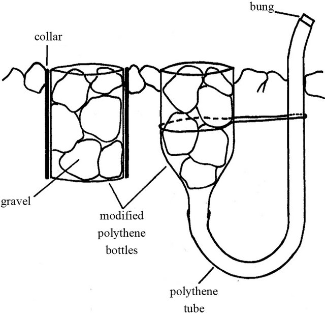
Reference [39] described an unmodified trap and a suction trap (Figure 2). Traps are not expected to give net rates of sedimentation, but to estimate the amount of material that will settle on a particular area. The unmodified trap was made from the bottom 90 mm section of a 500 ml polythene bottle with a diameter of 71 mm. A collar was made using an 80 mm diameter plastic drainpipe 120 mm in length. The drain pipe was buried and the trap was placed inside flush with the streambed. The trap was filled with clean gravel. The modified suction trap design was made from 120 mm of a 500 ml polythene bottle. Polythene pipe with a 22 mm inner diameter was wired to the neck of the bottle and bent in a U shape. The traps were buried flush with the streambed and filled with clean gravel. The polythene tube projected about 50 mm above the stream bed and the end was fitted with a bung. Each trap was emptied by sucking material from the U-tube with a pipe connected to a 1-liter evacuated flask.
 (a) (b)
Figure 2. An unmodified trap (a) and suction trap (b) constructed from polythene bottles [39].
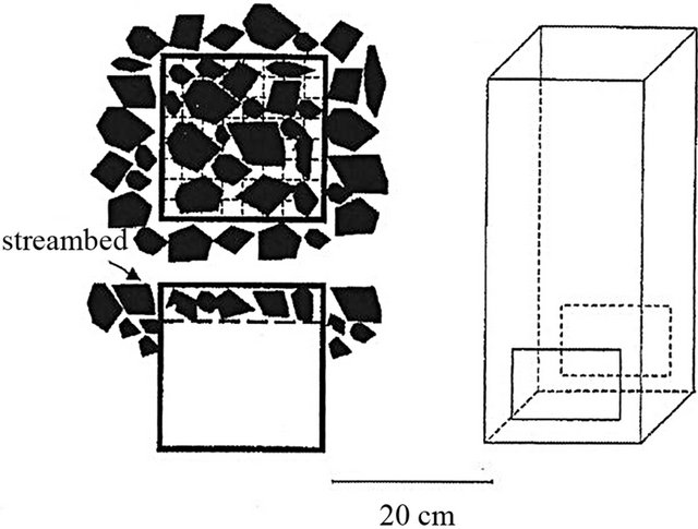
Reference [20] modified Whitlock-Vibert (W-V) boxes to use in trapping sediments (Figure 3). The boxes are typically used to incubate fish eggs in stream gravels. The boxes are made of polypropylene and measure 14 × 6.4 × 8.9 cm deep. The inner panels were removed and the boxes were filled with clean gravel 12 × 25 mm in diameter. A strip of duct tape was placed on the bottom. These boxes are buried in the stream sediment so that the tops are flush with the streambed. At the end of sampling, the whole box is removed from the substrate.
Reference [40] created another trapping device using two cylindrical containers with perforated walls. Two cylinders (one inside the other) are placed into the streambed with openings aligned. At retrieval, rotation of the inner container closes the device and prevents loss of fine material. This sampler is cost effective, and avoids the problem of sediment loss in W-V boxes [40] (Lanchance and Dube, 2004).
Reference [31] designed a sediment sampler with two parts, a base and a trap. The base was constructed from 10.16 cm schedule 40 PVC coupling with a height of 9.53 cm. The top half of the coupling was ground out using a 115 mm × 6 mm × 22.2 mm metal grinding wheel attached to a 0.33 hp, 1725 rpm, electric motor. This was done to allow the trap to slide freely in and out of the base. The trap was constructed by fitting (with silicon) a 10.16 cm insert cap onto a 5 cm piece of 10.16 cm schedule 40 PVC pipe (Figure 4).
During sampler deployment, the base was embedded in the substrate with the base top flush with the substrate. Next, the trap, filled with 12 - 25 mm diameter white gravel, was inserted into the base. At subsequent sampling events, the trap was removed and replaced, but the base remained embedded in the streambed. The two-part design allowed disturbance of the streambed only once at the onset of deployment, and prevented accidental addition or loss of sediment during deployment or retrieval. The white gravel that had been previously placed in the samplers were removed before analysis [31].
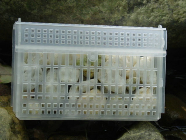
Figure 3. Whitlock-Vibert boxes to use in trapping sediments, introduced by Wesche et al. [20].
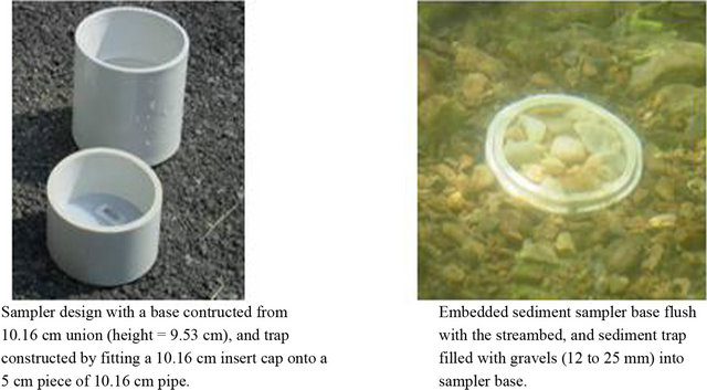
Figure 4. A two part trap design created by Hedrick et al. [31].
Reference [30] created a basic trap design made of simple plastic storage boxes (200 × 200 × 200 mm) available from most large hardware stores. Four holes (3 mm diameter) are drilled approximately 30 mm from the top of the trap so that two pieces of wire rod (3 mm dia. and 205 mm long) can be passed through the box. A piece of wire mesh (25 × 25 mm openings, 1.5 mm gauge wire), was cut to fit just inside the box, and was placed on top of these rods (Figure 5). The boxes are buried in the streambed and the wire mesh supports one layer of coarse bed material. This creates hydraulic conditions over the box similar to the rest of the streambed, but also creates conditions within the box that allow fine particles to settle. Sediment is collected using a tall open Perspex or plexiglass box that is large enough to fit around the trap. The box has two openings on opposite sides above the base. Attached to the downstream hole is a fine (60 μm) mesh net on a 170 mm frame passing through from the inside. The coarse substrate and wire mesh are removed and the sediment in the trap is resuspended and washed into the net. The traps can be left in situ for long-term monitoring [30].
Reference [41] created sediment traps that were similar to those described by Reference [30]. They used small plastic buckets as the collection container (depth 200 mm, radius 82.5 mm), providing a settlement area of 0.0213 m2. Once installed, traps were flush with the streambed and were covered with a layer of coarse substrate material, supported by wire mesh over the trap to minimize the alteration of hydraulic conditions [30]. Sediment was trapped for 24 hours.
The number of traps used varied. Reference [30] placed 5 traps at each sampling location of streams with average widths of 4 m. Sediment traps were placed in riffle areas. In a field testing experiment on the North Fork of the
 (a) (b)
Figure 5. A sediment trap and plastic column used to sample sediment from the trap [30].
Snake River, Reference [20] installed 12 modified W-V boxes at each study reach. Study reaches average 12 m in length and 6.5 m in width. Reference [31] also used 12 samplers each at sites located upstream and downstream of highway construction in an Appalachian stream. Average stream width varied from 5.5 - 8.2 m.
Sediments collected in sediment traps are most often returned to a laboratory where they are dried and sieved into size classes (30, 31, 20). Data can be analyzed by examining differences among size classes for traps located at different sampling sites, such as upstream and downstream, or on different streams that have similar flow environments [30].
2.4. Bedload Samplers
Bedload samplers can vary from small hand held units to large cable suspended units. These samplers are designed to sample sand, silt, gravel or rock debris carried by a stream on or immediately above its bed. These devices consist of an open metal body with a front intake nozzle through which water and sediment pass, and a flare that expands to the back of the sampler. The flare causes pressure differences within the sampler and encourages deposition in an attached bag. If flow resistance is created at the entrance of the sampler, some of the bedload material may accumulate in front of the sampler, causing the efficiency of the sampling device to vary. A pressure difference sampler ensures that the intake velocity and stream velocity are identical [42]. All pressure-difference samplers have this same basic configuration, different versions have openings and flares of varying sizes. Samplers are typically constructed of sheet metal, metal plates, or cast aluminum, which provide varying thickness to the walls. All pressure-difference samplers may be hand-held and used while wading or deployed from small bridges, or suspended from cables and held in place using staylines.
The most commonly used pressure-difference sampler is the original Helley-Smith bedload sampler (Figure 6). The sampler had a square entrance nozzle (76 × 76 mm), a frame with fins for stabilization, and a sample bag constructed of 0.25 mm-mesh polyester [43]. The sampler had an expansion ratio (exit area/entrance area) of 3.22. A hand held version of the sampler has been used in wadeable streams (Figure 7) [44,45]. The length and stability of the handle is important and those made of galvanized steel or aluminum tubing work best [46].
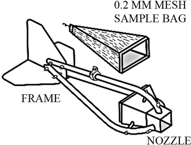
Figure 6. Schematic of the Helley-Smith bedload sampler.
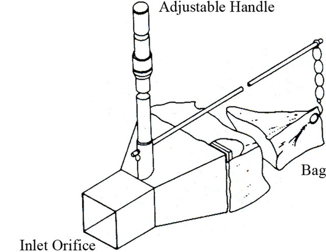
Figure 7. Schematic of wading bedload sampler.
Several different versions of the sampler have been designed and used for various field conditions [47]. Reference [48] created a similar sampler (BLH-84) that had a smaller expansion ratio of 1.4. This design makes it easier to fit the sampler into a rocky stream bottom. Reference [35] used a modified version of this sampler with a larger opening of 152 mm in proglacial streams in Switzerland. Reference [49] made bed load measurements with hand held pressure difference sampler that had a sampler opening measuring 0.3 × 0.15 m. The expansion ratio was 1.4, and the sampler was equipped with a 0.25 mm mesh bag. The dimensions of this sampler were similar to the Toutle River sampler designed by Reference [47]. The Toutle River sampler has a rectangular shaped intake of 0.15 × 0.3 m, and a 1.4 expansion ratio, and is made from a 0.64 cm steel plate [47].
Reference [50] modified the trap to catch coarse gravel and small cobble. The aluminum frame was built 0.3 m wide at the sampler opening. The 0.9 m trailing net with 3.6 mm mesh is designed to be opened and emptied from the back without removing the frame from the streambed. Bedload traps were placed on 0.3 by 0.41 m ground plates that are anchored to the stream bottom with metal stakes. Adjustable nylon webbing straps are used to fasten the frame to the stakes (Figure 8).
Reference [45] studied 19 gravel bed mountain stream channels to relate patterns of transport to basin and channel characteristics. They used two different types of bedload samplers depending on the stream size. At most sites the hand held Helley Smith bedload sampler (76 × 76 mm) was used. Samples from four streams were collected using a wading version of the Elwha bedload sampler with a 102 × 203 mm opening [47]. The Elwha sampler is a scaled-down version of the Toutle River sampler, with a smaller opening and a similar flare and expansion ratio [51]. The rectangular shape helped stabilize the larger sampler on the stream bottom; however, the increased
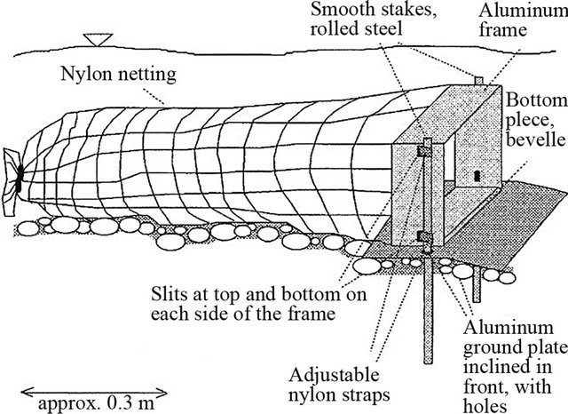
Figure 8. A modified bedload trap with plate [50].
size and mass do make the samplers more challenging to handle at high flows [45].
The number of samples collected varies depending on stream width and research interests. Reference [52] suggested sampling a minimum of 20 equally-spaced points per traverse, with two traverses made per bedload sample. With this approach, about 40 vertical measurements comprise one sample. This number of verticals is probably excessive in small mountain streams, because channels are typically narrower and the sampler occupies a larger proportion of the streambed, so fewer verticals are needed to achieve a suitable spatial measurement [45]. Reference [50] suggested that the width of all traps cover 20% - 40% of the active streambed. This varied from 5 to 6 traps for the larger modified samplers and 12 - 18 for the smaller Helley Smith sampler. The US Geological Survey recommends a sampling time of 30 - 60 seconds for each vertical in gravel-bed streams, Reference [45] suggested 1 - 2 minutes in cobble and boulder-bed channels. Reference [35] collected 3 - 10 verticals per transverse and each vertical sampler was deployed for 30 sec. Samples varied in weight from 0.0005 - 13.31 kg.
Bedload samples are normally dried and sieved using standard sedimentological methods. Full phi-interval sieves, ranging from 0.5 - 64 mm can be used [35,45,49].
The fraction of each sediment class per sample can be used to examine changes in sediment over time. Data can also be used to analyze transport rates.
Bedload samplers can be purchased commercially from a variety of sources. A 1.8 kg Helley Smith Hand Held Sampler with a 0.76 mm opening can be purchased from Forestry Suppliers (www.forestry-suppliers.com). The Rickly Hydrological Company (www.rickly.com) sells a variety of samplers including the handheld Helley Smith, the BLH-84, and the Toutle River sampler.
2.5. Freeze Core
Freeze core samplers are designed to collect vertical profiles of streambed substrate. Samplers consist of one or more hollow rods with a pointed tip and can be constructed of cooper [53] or stainless steel [54] tubing. The rod is driven approximately 0.2 m into the streambed with a deadblow hammer and is then injected with either carbon dioxide or liquid nitrogen by a 9-kg capacity fire extinguisher (Figure 9). The gas escapes through nozzles at the lower end of each rod. Pore water in the sediment adjacent to the rod freezes, and the frozen core is extracted from the streambed for analysis. Freeze cores typically weigh from 1 - 5 kg when sampled with liquid
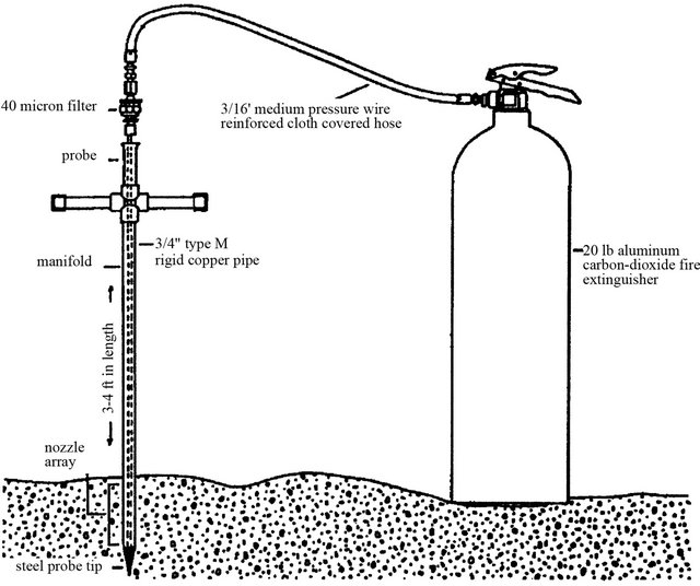
Figure 9. Freeze core sampler.
carbon dioxide, and 10 - 15 kg when sampled with liquid nitrogen [55]. Reference [54] created a probe template to hold three probes in a triangular array. The template is constructed from two circular steel plates mounted on a threaded steel rod.
A major advantage of the freeze-core sampler is that it provides opportunity for vertical stratification of substrate cores. The stratification of bed-material remains intact, unlike the homogenization of streambed material that occurs when the streambed is sampled with a core sampler [56]. One disadvantage is that the stratification of the bed material may be disturbed as fine sediment is shaken deeper into the bed during the pounding of the rods into the bed [56]. A second disadvantage is the irregular shapes of freeze core samples, depending on how far the freezing advanced outward from the rod. Large particles that are only partially frozen to the core may loosen during rod retrieval, or a few large particles may also be frozen to the rod and dominate the sample, causing an under representation of fine sediment [27,53].
Reference [27] used a modified version of the single probe system [53]. They used steel conduit (2.2 cm outside diameter, 76 cm long) with a solid conical point at the bottom end, driven into the streambed to a target depth of 26 cm. Reference [27] compared these to excavation core samples and shovel samples. The freeze core sampler produced the smallest sample; however, it was the most complex and expensive of the three devices. The freeze core sampler collected more fines (<0.212 mm), however, it also collected more particles over 50 mm. More fine particles were found in the lower half of the freeze core sample.
2.6. Pebble Count
The Wolman pebble count [57] is the most common method used for conducting in stream measurements of sediment. Wolman’s original method was created for wadeable rivers flowing over coarse material. Wolman suggested placing a transect across the stream and measuring 100 individual pebbles from the bed. The sampler should try not to look at the streambed when choosing the particle. Each particle is drawn from under the toe of the samplers boot. The intermediate axis of each pebble is measured. The principal limitations of this method are the inability to accurately measure fine particles in the field, and difficulty in measuring in deep water [57].
A well established method, the “Wolman Pebble Count” has been used and varied by researchers to characterize stream bed sediment size classes [18,58-61]. Another option to choosing a particle beneath the boot toe is to use the finger tip method. A fixed point on the tip of the finger is used to select the particle for measurement [18]. A staff or 0.32 cm welding rod can also be used to determine which particle to choose. If the staff hits fine sediment that covers a rock it should be counted as fines not the rock. A person can tell if they hit fines because the rod will make a “scrunch” or “squish” sound rather than a solid “thunk” [62].
The number of transects sampled depends on the researchers interest. Reference [58] took measurements at 10 equally spaced transects in each study reach. Reference [63] made 100 pebble measurements at three to four locations along a 100 m stream reach. Due to fast and deep flows at some of their sampling locations, Reference [61] modified the transect method and used a 3 × 3 m section of streambed. At each location a minimum of 100 particles (mean = 120, range = 100 - 219) were sampled. Reference [60] used a 400 pebble count method. At each reach, transects were randomly located across riffles. If four riffles were present 100 counts were made per transect. If fewer were present the count was evenly spread out among the riffles that are present using the same four-transect setup (e.g., if two riffles are present, each will have a 200 particle count). Within each riffle, four transects were spaced at 20%, 40%, 60%, and 80% of the riffle length.
Particles are measured and tallied using the Wentworth size classes (Table 1). The intermediate axis of each particle is measured. This is neither the longest nor shortest of three mutually perpendicular axes of a particle, and is the axis which controls whether or not it would pass through a soil sieve [18]. Particles can be measured using a ruler or calipers. A gravelometer, a thin aluminum or plastic template with square sieve size holes can also be used [50,60,64]. Templates are preferred to ruler and calipers because of the potential to improperly measure the particle and read the instrument.
Once the particles are tallied, the cumulative percent finer is calculated for each size class, and the data are plotted as a cumulative size distribution curve. The frequency distribution represents the percent of the streambed covered by particles of a certain size, since each pebble represents a portion of the bed surface. Results are theoretically equivalent to size distributions obtained from bulk samples of substrate surface materials. Data are plotted as cumulative frequency curves and interpreted with respect to the percent of the bed surface covered by particles finer than a predetermined size of significance. Pebble counts can help detect increases in fine sediment under certain circumstances [18].
Reference [65] focused on difference in % fines as calculated from particle sizes at 21 evenly spaced cross sections per site. Five particles were selected per cross section. For sand and finer particles, field crews determined the dominant size class from a pinch of fine particles. Percent fines were classified as <0.06 mm and % sand and fines were <2 mm. Because the collection points were systematically spaced, Reference [65] interpreted these percentiles as surficial areal estimates of the substrate characteristics of each sampled stream reach.
2.7. Cross Section
Surveying the cross-section of a stream channel can give a representation of the geology of the channel and if surveyed over an extended period of time can show the change in channel morphology. A stream channel cross section is a series of measurements along a permanently established transect across the width of the stream. Distance and elevation readings are taken at intervals across the transect, including bankfull, edge of water, thalweg, and any bar formations. At each cross section, a permanent marker is established on a stable site above the bankfull channel, and elevations are referenced to the local benchmark. Changes over time in cross sections determine vertical stability of the streambed, and indicate sedimentation. The change in cross-sectional area can be determined as scour or degradation (a negative value) or as fill or aggradation (a positive value).
The number of cross sections and how often they are monitored will vary depending on research objectives. Reference [66] surveyed 30 cross sections at an upstream reach of Oyabu Creek, a headwater stream located in southern Japan and 70 cross sections downstream of Oyabu Creek with the confluence of Kochino-tai tributary. The area was affected by typhoons in 1993, 1997 and heavy rainfall in 1999. Reference [35] monitored changes in cross sections at three sites on a daily basis during their study of a proglacial meltwater stream in Valais, Switzerland. They also surveyed 28 monumented cross sections spaced at 9-m intervals twice during their year study period. Reference [67] established four cross sections, two across a reference reach and two across a reach altered by highway construction. The cross sections were surveyed four times in a four-year period.
Cross section measurements do not indicate changes in the sediment size of the streambed and are often used in conjunction with other sampling measurements in studies related to streambed sedimentation. Reference [35] also took sediment samples using the shovel method and a modified Helley-Smith sampler. In their study on highway construction, Reference [31] monitored sedimentation in the same stream reach as cross sectional surveys using sediment traps.
2.8. Grid Toss and Visual Estimation
Visual estimation of sediment coverage on the streambed can be done within a specified area of the streambed [41, 63] or by use of a grid toss [68,69]. The standard size grid is 0.30 m2 and the intersection size is approximately 6 mm [69]; (Figure 10). There are 49 “internal” intersec-
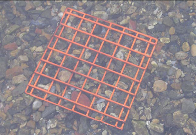
Figure 10. A standard size grid (approximately 0.30 m2) used in the “grid toss” evaluation of fine sediment [69].
tions. The grid is randomly “tossed” in each zone sequentially. Zones are located at approximately at 25%, 50% and 75% of the wetted channel width. The grid can break if it lands on an edge, so the “toss” should be made gently and the grid should land on the channel bed relatively flat. To assess the percent of fine sediment <6 mm, the number of intersections that “cover” (or intersect with) particles <6 mm are counted. Intersections along the edge of the grid are not counted [69].
Reference [63] estimated percent deposited sediment to the nearest 5% by visually examining the streambed substrate content within a 0.5 m2 metal frame placed upon the streambed. A value of 1% was recorded in the case where deposited sediment was less than 5% but greater than 0%. Percent deposited sediment was substrate sizes < 2 mm.
Reference [41] estimated the percentage of substrate covered by fine sediment within a 300 mm wide strip across the width of the stream at 15 cross sections on three occasions. From these measurements, they calculated an average percentage cover of fine sediment for each reach and time. They found reducing stream flow on three small New Zealand streams increased sediment coverage.
3. Analysis Methods
Sample processing can be done on wet or dry samples. Volumetric sampling can be done on wet samples with standard equipment and methods by washing the samples through a set of nested sieves. Reference [32] suggested sieve sizes with openings (in mm) of 75.0, 25.0, 9.5, 3.35, 2.0, 1.0, 0.85, 0.50, 0.25, and 0.106. Wash water and particles washed through the 0.106 mm sieve are collected in a catch basin. The sample should be allowed to settle out for 20 minutes so particles can be collected in a graduated cylinder attached to the bottom of the catch basin. Once the cylinder is removed and the material has settled, a volume reading is made. Sieves are drained for 15 minutes. The volume of each sieve can be measured by placing the contents in a displacement flask and recording the volume of the displaced water [28].
Sediment from gravel-bed rivers can also be dried before sieving. Samples should settle undisturbed for 48 hours, and then excess water should be carefully siphoned off to within 5 cm of the gravel layer. Wet sediment can be dried on metal pans for two or three days with exposure to air at room temperature, or in a drying oven at 90˚C (194˚F) overnight. Particles should be allowed to cool to room temperature before sieving and weighing to avoid measuring an increase in particle weight as the particle absorbs air moisture during the cooling phase. The gravel from one or more pans is poured into the set of nested sieves that has a sieve pan at the bottom. The amount of sediment that can be sieved at a time depends on the number of sieves used and on the particle sizes. Sieves are mounted on a shaker, a sieving apparatus that automatically shakes the sieve stack. After the sample is shaken, each sieve should be brushed thoroughly before measuring the material collected [50]. The particle sievesize can be defined as the smallest sieve size through which a particle can pass or as the largest sieve size through which the particle did not pass, called the retaining sieve size [60]. Sediment in each size class can be weighed, or can be measured by water displacement and expressed as a volumetric proportion of the whole substrate sample [25].
Reference [18] detailed two general methods to describe the particle size distribution of samples. The first relies on quantifying the proportion of bed material particles less than a given size by weight or volume. Definitions of fines for this purpose ranged from 0.74 mm to 8 mm. The second approach quantifies bed material particles as some measure of central tendency. Expressions of central tendency for the particle size included the arithmetic mean, the geometric mean, and the median. The total mass and median particle size (by mass) can be determined for each sample. A particle-size frequency and a percentage frequency distribution can be computed from these measurements. A cumulative frequency distribution can also be computed. Percentiles can be determined from the cumulative distribution curve and can be used when comparing D50 sizes. The D50 size is the particle diameter associated with the 50th percentile class of the particle cumulative frequency distribution for each sediment sample. Percentiles can also be used to derive particle-distribution parameters such as mean and standard deviation [50].
4. Summary
Monitoring the streambed particle size distribution can be useful in studies that are monitoring watershed impacts and changes in stream habitat. The amount of fine sediment in a streambed habitat can have impacts on stream biota. Multiple methods exist for collecting samples that can be analyzed in the lab, and for conducting on-site evaluations of sediment size distributions. Sediment samples can be collected using core sampling techniques, the shovel method, sediment traps, bedload samplers, and freeze core samplers. On-site evaluations can be conducted using pebble count methods, surveying cross sections of a stream, a grid toss, and visual estimation. The method or methods chosen by researchers will vary on location of study sites, proximity of sites to road access, the goals of the research, and laboratory time and equipment available.
Core samplers, freeze core samplers, and shovel methods disturb a portion of the streambed and are most useful for single or annual use. Freeze core samples provide a vertical profile of the streambed substrate and can be useful for research analyzing streambed layers. Sediment traps can be used for repeated measures over time, and create smaller samples than shovel and core samplers. These are useful when collecting large numbers of samples, or sampling in remote locations. Bedload samplers are commercially available and can be a variety of sizes. These samplers must be hand held or anchored in the stream for the duration of the sampling event, which may last from 30 - 120 seconds. Sediment samples collected by these methods are most often returned to the lab for processing through sieves using either wet or dry methods.
The Wolman pebble count is a popular method of characterizing the streambed surface particles. It requires little sampling gear and multiple teams can be used at a location to limit the time necessary. After data are collected, percent fines and dominant size classes can be calculated. Visual estimation of sediment coverage can be done using a grid, along a transect, or within a set area of a metal frame. This method is useful for assessing the percent of fine sediment. Cross sectional surveys do not characterize the streambed but can be used to identify streambed aggradation and degradation, and are useful in conjunction with other methods to identify streambed changes.
In conclusion, researchers interested in evaluating streambed sediments over time or characterizing the streambed sediment particle sizes can choose to use a variety of techniques. Methods are available for annual or one-time samples and continuous samples over time. Samples can be collected and returned to the lab for processing and changes in the percent fines or differences in percent fines per location can be compared. It is important for researchers to evaluate different methods available and choose the ones most useful to their research interest and sampling locations.
5. Acknowledgements
We thank the West Virginia Division of Highways for providing partial support for this research. Jim Hedrick and Frank Jernejcic of the West Virginia Division of Natural Resources provided valuable reviews and comments. Reference to trade names does not imply endorsement of commercial products by the US government. This is scientific article number 3147 of the West Virginia University Agriculture and Forestry Experimental Station.
REFERENCES
- R. D. Judy Jr., P. N. Seely, T. M. Murray, S. C. Svirsky, M. R. Whitworth and L. S. Ischinger, “National Fisheries Survey, Volume I. Technical Report: Initial Findings,” US Fish and Wildlife Service, Washington DC, 1982.
- United States Environmental Protection Agency, “National Water Quality Inventory: 1988 Report to Congress,” EPA Report 440490003, Washington DC, 1990.
- B. D. Richter, D. P. Braun. M. A. Mendelson and L. L. Master, “Threats to Imperiled Freshwater Fauna,” Conservation Biology, Vol. 11, No. 5, 1997, pp. 1081-1093. doi:10.1046/j.1523-1739.1997.96236.x
- United States Environmental Protection Agency, “National Water Quality Inventory: 1992 Report to Congress,” EPA Report 841R94001, Washington DC, 1994.
- P. J. Wood and P. D. Armitage, “Biological Effects of Fine Sediment in the Lotic Environment,” Environmental Management, Vol. 21, No. 2, 1997, pp. 203-217. doi:10.1007/s002679900019
- S. Entrekin, M. Evans-White, B. Johnson and E. Hagenbuch, “Rapid Expansion of Natural Gas Development Poses a Threat to Surface Waters,” Frontiers in Ecology and the Environment, Vol. 9, No. 9, 2011, pp. 503-511. doi:10.1890/110053
- T. F. Waters, “Sediment in Streams: Sources, Biological Effects, and Control,” Monograph 7, American Fisheries Society, Bethesda, 1995.
- M. A. Brusven and K. V. Prather, “Influence of Stream Sediment on Distribution of Macrobenthos,” Journal of Entomological of Society British Columbia, Vol. 71, No. 1, 1974, pp. 25-32.
- D. A. Lemly, “Modification of Benthic Insect Communities in Polluted Streams: Combined Effects of Sedimentation and Nutrient Enrichment,” Hydrobiologia, Vol. 87, No. 3, 1982, pp. 229-245. doi:10.1007/BF00007232
- J. W. Burns, “Some Effects of Logging and Associated Road Construction on Northern California Streams,” Transactions of the American Fisheries Society, Vol. 101, No. 1, 1972, pp. 1-16. doi:10.1577/1548-8659(1972)101<1:SEOLAA>2.0.CO;2
- G. Lamberti and M. B. Berg, “Invertebrates and Other Benthic Features as Indicators of Environmental Change in Juday Creek, Indiana,” Natural Areas Journal, Vol. 15, No. 3, 1995, pp. 249-258.
- K. Wentworth, “A Scale of Grade and Class Terms for Clastic Sediments”, Journal of Geology, Vol. 30, No. 5, 1922, pp. 377-392. doi:10.1086/622910
- L. Fraley, “Methods of Measuring Fluvial Sediment,” Center for Urban Environmental Research and Education, University of Maryland, Baltimore, 2004.
- D. W. Chapman, “Critical Review of Variables Used to Define Effects of Fines in Redds of Large Salmonids,” Transactions of the American Fisheries Society, Vol. 117, No. 1, 1988, pp. 1-21. doi:10.1577/1548-8659(1988)117<0001:CROVUT>2.3.CO;2
- D. A. Hausle and D. W. Coble, “Influence of Sand in Redds on Survival and Emergence of Brook Trout (Salvelinus fontinalis),” Transactions of the American Fisheries Society, Vol. 105, No. 1, 1976, pp. 57-63. doi:10.1577/1548-8659(1976)105<57:IOSIRO>2.0.CO;2
- D. G. Argent and P. A. Flebbe, “Fine Sediment Effects on Brook Trout Eggs in Laboratory Streams,” Fisheries Research, Vol. 39, No. 3, 1999, pp. 253-262. doi:10.1016/S0165-7836(98)00188-X
- J. P. Hakala, “Factors Influencing Brook Trout (Salvelinus fontinalis) Abundance in Forested Headwater Streams with Emphasis on Fine Sediment,” M.S. Thesis, West Virginia University, Morgantown, 2000.
- J. P. Potyodony and T. Hardy, “Use of Pebble Counts to Evaluate Fine Sediment Increase in Stream Channels,” Water Resources Bulletin, Vol. 30, No. 3, 1994, pp. 509- 520. doi:10.1111/j.1752-1688.1994.tb03309.x
- P. R. Kaufmann, P. Levine, E. G. Robinson, C. Seeliger and D. V. Peck, “Quantifying Physical Habitat in Wadeable Streams EPA/620/R-99/003,” US Environmental Protection Agency, Washington DC, 1999.
- T. A. Wesche, D. W. Reiser, V. R. Hasfurther, W. A. Hubert and Q. D. Skinner, “New Technique for Measuring Fine Sediment in Streams,” North American Journal of Fisheries Management, Vol. 9, No. 2, 1989, pp. 234-238. doi:10.1577/1548-8675(1989)009<0234:NTFMFS>2.3.CO;2
- United States Environmental Protection Agency, “Quality Criteria for Water 1986, EPA 440/5-86-001,” Office of Water Regulations and Standards, Washington DC, 1996.
- R. L. Beschta, “Suspended Sediment and Bedload,” In: F. R. Hauer and G. A. Lambert, Eds., Methods in Stream Ecology, Academic Press, San Diego, 1996, pp. 123-144.
- United States Environmental Protection Agency, “Monitoring Water Quality, EPA 841-B-97-003,” Office of Water Regulations and Standards, Washington DC, 1997.
- W. F. McNeil and W. H. Ahnell, “Success of Pink Salmon Spawning Relative to Size of Spawning Bed Materials,” US Fish and Wildlife Service Special Scientific Report—Fisheries Number 469, Washington DC, 1964.
- W. S. Platts, R. J. Torquemada, M. L. McHenry and C. K. Graham, “Changes in Salmon Spawning and Rearing Habitat from Increased Delivery of Fine Sediment to the South Fork Salmon River, Idaho,” Transactions of the American Fisheries Society, Vol. 118, No. 3, 1989, pp. 274-283. doi:10.1577/1548-8659(1989)118<0274:CISSAR>2.3.CO;2
- J. C. Wellman, D. L. Combs and S. B. Cook, “Long-Term Impacts of Bridge and Culvert Construction or Replacement on Fish Communities and Sediment Characteristics of Streams,” Journal of Freshwater Ecology, Vol. 15, No. 3, 2000, pp. 317-328. doi:10.1080/02705060.2000.9663750
- R. T. Grost, W. A. Hubert and T. A. Wesche, “Field Comparison of Three Devices Used to Sample Substrate in Small Streams,” North American Journal of Fisheries Management, Vol. 11, No. 3, 1991, pp. 347-351. doi:10.1577/1548-8675(1991)011<0347:FCOTDU>2.3.CO;2
- D. S. Hames, B. Conrad, A. Pleus and D. Smith, “Field Comparison of the McNeil Sampler with Three ShovelBased Methods Used to Sample Spawning Substrate Composition in Small Streams,” Northwest Indian Fisheries Commission TFW Ambient Monitoring Program Report, 1996.
- G. S. Eaglin and W. A. Hubert, “Effects of Logging and Roads on Substrate and Trout in Streams of the Medicine Bow National Forest, Wyoming,” North American Journal of Fisheries Management, Vol. 13, No. 4, 1993, pp. 844-846. doi:10.1577/1548-8675(1993)013<0844:MBEOLA>2.3.CO;2
- N. R. Bond, “A Simple Device for Estimating Rates of Fine Sediment Transport along the Bed of Shallow Streams,” Hydrobiologia, Vol. 468, No. 1-3, 2002, pp. 155-161. doi:10.1023/A:1015270824574
- L. B. Hedrick, S. A. Welsh and J. D. Hedrick, “A New Sampler Design for Measuring Sedimentation in Streams,” North American Journal of Fisheries Management, Vol. 25, No. 1, 2005, pp. 238-244. doi:10.1577/M03-236.1
- D. Schuett-Hames, R. Conrad, A. Pleus and M. Henry, “TFW Monitoring Program Method Manual for the Salmonid Spawning Gravel Composition Survey,” Department of Natural Resources under the Timber, Fish, and Wildlife Agreement, Washington DC, 1999.
- M. Christensen, A. Nakajima and A. Baun, “Toxicity of Water and Sediment in a Small Urban River (Store Vejlea, Denmark),” Environmental Pollution, Vol. 144, No. 2, 2006, pp. 621-625. doi:10.1016/j.envpol.2006.01.032
- J. Muskatirovic, “Analysis of Bedload Transport Characteristics of Idaho Streams and Rivers,” Earth Surface and Landforms, Vol. 33, No. 11, 2008, pp. 1757-1768. doi:10.1002/esp.1646
- J. Warburton, “Observations of Bed Load Transport and Channel Bed Changes in a Proglacial Mountain Stream,” Artic and Alpine Research, Vol. 24, No. 3, 1992, pp. 195- 203. doi:10.2307/1551657
- H. E. Berkman and C. F. Rabeni, “Effects of Siltation on Stream Fish Communities,” Environmental Biology of Fishes, Vol. 18, No. 4, 1987, pp. 285-294. doi:10.1007/BF00004881
- R. B. Painter, “The Measurement of Bed Load Movement in Rivers,” Journal of Water Resources and Environmental Engineering, Vol. 76, 1972, pp. 291-294.
- T. E. Lisle, “Sediment Transport and Resulting Deposition in Spawning Gravels, North Coastal California,” Water Resources Research, Vol. 25, No. 6, 1989, pp. 1303- 1319. doi:10.1029/WR025i006p01303
- J. S. Welton and M. J. H. Ladle, “Two Sediment Trap Designs for Use in Small Rivers and Streams,” Limnology and Oceanography, Vol. 24, No. 3, 1979, pp. 588-592.
- S. Lachance and M. Dube, “A New Tool for Measuring Sediment Accumulation with Minimal Loss of Fines,” North American Journal of Fisheries Management, Vol. 24, No. 1, 2004, pp. 303-310. doi:10.1577/M02-087
- Z. D. Dewson, A. B. W. James and R. G. Death, “Stream Ecosystem Functioning under Reduced Flow Conditions,” Ecological Applications, Vol. 17, No. 6, 2007, pp. 1797-1808. doi:10.1890/06-1901.1
- W. H. Graf, “Hydraulics of Sediment Transport,” Water Resources Publications, LLC, Highlands Ranch, 1994.
- E. J. Helley and W. Smith, “Development and Calibration of a Pressure-Difference Bedload Sampler,” US Geological Survey Open-File Report 8037-01, 1971, 18 p.
- S. E. Ryan and W. W. Emmet, “The Nature of Flow and Sediment Movement in Little Granite Creek near Bondurant, Wyoming,” General Technical Report RMRS-GTR- 90, US Department of Agriculture, Forest Service, Rocky Mountain Research Station, Ogden, 2002, 48 p.
- S. E. Ryan, L. S. Porth and C. A. Troendle, “Coarse Sediment Transport in Mountain Streams in Colorado and Wyoming, USA,” Earth Surface Processes and Landforms, Vol. 30, No. 3, 2005, pp. 269-288. doi:10.1002/esp.1128
- S. E. Ryan and C. A. Troendle, “Measuring Bedload with Handheld Samplers in Coarse-Grained Mountain Channels,” Streams Systems Technology Center, Rocky Mountain Research Station, Fort Collins, 1999, 8 p.
- D. Childers, “Field Comparisons of Six Pressure-Difference Bedload Samplers in High-Energy Flow,” US Geological Survey Water-Resources Investigations Report 92-4068, 1999, 59 p.
- D. W. Hubbell, H. H. Stevens, J. V. Skinner and J. P. Beverage, “Recent Refinements in Calibrating Bedload Samplers,” Water Forum 81, American Society of Civil Engineers, New York, Vol. 1, 1981, pp. 128-140.
- Y. Lui, F. Metivier, J. Gaillardet, B. Ye, P. Meunier, C. Narteau, E. Lajeunesse, T. Han and L. Malverti, “Erosion Rates Deduced from Seasonal Mass Balance along an Active Braided River in Tianshan,” Solid Earth Discussion, Vol. 3, 2011, pp. 541-589. doi:10.5194/sed-3-541-2011
- K. Bunte, S. R. Abt, J. P. Potyondy and S. E. Ryan, “Measurement of Coarse Gravel and Cobble Transport Using Portable Bedload Traps,” Journal of Hydraulic Engineering, Vol. 130, No. 9, 2004, pp. 879-893. doi:10.1061/(ASCE)0733-9429(2004)130:9(879)
- D. Childers, D. L. Kresch, S. A. Gustafson, T. J. Randle, J. T. Melena and B. Cluer, “Hydrologic Data Collected during the 1994 Lake Mills Drawdown Experiment, Elwha River, Washington,” US Geological Survey, Water Resources Investigation Report 99-4215, 2000.
- W. W. Emmett, “Measurement of Bedload in Rivers,” Erosion and Sediment Transport Measurements IAHS Publication No. 133, Proceedings of the Florence Symposium, June 1981, 13 p.
- W. J. Walkotten, “An Improved Technique for Freeze Sampling Streambed Sediments,” US Forest Service Research Note PNW-281, Pacific Northwest Forest and Range Experiment Station, Portland, 1976, 11 p.
- F. H. Everest, C. E. McLemore and J. F. Ward, “An Improved Tri-Tube Cryogenic Gravel Sampler,” US Forest Service Research Note PNW-350, Pacific Northwest Forest and Range Experiment Station, Portland, 1980, 6 p.
- K. Bunte and S. R. Abt, “Sampling Surface and Subsurface Particle-Size Distributions in Wadable Gravel and Cobble-Bed Streams for Analyses in Sediment Transport, Hydraulics, and Streambed Monitoring,” General Technical Report RMRS-GTR-74, US Department of Agriculture, Rocky Mountain Research Station, Fort Collins, 2001.
- T. E. Lisle and R. E. Eads, “Methods to Measure Sedimentation of Spawning Gravels,” Research Note PSW-411, United States Department of Agriculture, Forest Service, Pacific Southwest Research Station Berkley, Albany, 1991.
- M. G. Wolman, “A Method of Sampling Coarse RiverBed Material,” Transactions, American Geophysical Union, Vol. 35, No. 6, 1954, pp. 951-956. doi:10.1029/TR035i006p00951
- K. J. Collier and J. M. Quinn, “Land-Use Influences Macroinvertebrate Community Response Following a Pulse Disturbance,” Freshwater Biology, Vol. 48, No. 8, 2003, pp. 1462-1481. doi:10.1046/j.1365-2427.2003.01091.x
- L. A. Golden and G. S. Springer, “Channel Geometry, Median Grain Size, and Stream Power in Small Mountain Streams,” Geomorphology, Vol. 78, No. 1-2, 2006, pp. 64-76. doi:10.1016/j.geomorph.2006.01.031
- [61] P. Kusnierz and A. Welch, “The Montana Department of Environmental Quality Sediment Assessment Method: Considerations, Physical and Biological Parameters, and Decision Making,” Montana Department of Environmental Quality, Helena, 2011.
- [62] H. J. Moi and G. B. Pasternack, “Relationships between Mesoscale Morphological Units, Stream Hydraulics and Chinook Salmon (Oncorhynchus tshawytscha) Spawning Habitat on the Lower Yuba River, California,” Geomorphology, Vol. 100, No. 3-4, 2008, pp. 527-548. doi:10.1016/j.geomorph.2008.02.001
- [63] G. M. Kondolf, “Application of the Pebble Count: Reflections on Purpose, Method, and Variants,” Journal of the American Water Resources Association, Vol. 33, No. 1, 1997, pp. 79-87. doi:10.1111/j.1752-1688.1997.tb04084.x
- [64] S. D. Longing, “Ecological Studies of Benthic Macroinvertebrates for Determining Sedimentation Impacts in Chattahoochee National Forest Streams,” Doctoral Dissertation, Virginia Polytechnic Institute and State University, Blacksburg, 2006.
- [65] K. Bunte, K. W. Swingle and S. R. Abt, “Guidelines for Using Bedload Traps in Coarse-Bedded Mountain Streams: Construction, Installation, Operation, and Sample Processing,” Stream Notes, Rocky Mountain Research Station, Fort Collins, 2007.
- [66] S. A. Bryce, G. A. Lomnicky and P. R. Kaufmann, “Protecting Sediment-Sensitive Aquatic Species in Mountain Streams through the Application of Biologically Based Streambed Criteria,” Journal of the North American Benthological Society, Vol. 29, No. 2, 2010, pp. 657-672. doi:10.1899/09-061.1
- [67] M. Kasai, T. Marutani and G. Brierley, “Channel Bed Adjustments Following Major Aggradation in a Steep Headwater Setting: Findings from Oyabu Creek, Kyushu, Japan,” Geomorphology, Vol. 62, No. 3-4, 2004, pp. 199- 215. doi:10.1016/j.geomorph.2004.03.001
- [68] L. B. Hedrick, S. A. Welsh and J. T. Anderson, “Influences of High Flow Events on a Stream Channel Altered by Construction of a Highway Bridge—A Case Study,” Northeastern Naturalist, Vol. 16, No. 3, 2009, pp. 375- 394. doi:10.1656/045.016.n306
- [69] J. D. Heitke, E. J. Archer, D. D. Dugaw, B. A. Bouwes, E. A. Archer, R. C. Henderson and J. L. Kershner, “Effectiveness Monitoring for Streams and Riparian Areas: Sampling Protocol for Stream Channel Attributes,” PACFISH/ INFISH Biological Opinion Effectiveness Monitoring Program (PIBO-EMP) Staff Multi-federal Agency Monitoring Program, Logan, 2006, 54 p.
- [70] J. L. Kershner, E. K. Archer, M. Coles-Rithchie, E. R. Cowley, R.C. Henderson, K. Kratz, C. M. Quimby, D. L. Turner, L. C. Ulmer and M. R. Vinson, “Guide to Effective Monitoring of Aquatic and Riparian Resources,” General Technical Report RMRS-GTR-121, US Department of Agriculture, Rocky Mountain Research Station, Fort Collins, 2004, 57 p.