Open Journal of Modern Hydrology
Vol.3 No.4(2013), Article ID:38963,9 pages DOI:10.4236/ojmh.2013.34030
On Redefining the Onset of Baseflow Recession on Storm Hydrographs
![]()
1University of Talca, Centro Tecnológico de Hidrología Ambiental, Talca, Chile; 2Department of Hydrology and Water Resources, University of Arizona, Tucson, Arizona; 3Instituto Forestal de Chile, Santiago, Chile; 4Dirección General de Aguas, Santiago, Chile.
Email: pablogarciach@gmail.com
Copyright © 2013 R. Pizarro-Tapia et al. This is an open access article distributed under the Creative Commons Attribution License, which permits unrestricted use, distribution, and reproduction in any medium, provided the original work is properly cited.
Received May 24th, 2013; revised June 24th, 2013; accepted July 2nd, 2013
Keywords: Baseflow Recession; Hydrograph Separation; Hydrologic Modeling; Recession Analysis; Baseflow Onset
ABSTRACT
Two methods that define the point of baseflow recession onset were compared using storm hydrograph data for 27 storm events that occurred between 1982-1995 in the Upeo watershed located in the Andes mountain range in central Chile (Figure 1). Three well-known baseflow recession equations were used to determine whether the method we are proposing here, that defines baseflow recession onset as the third inflection point on the logarithmic graph of the falling limb of the storm hydrograph, more accurately models observed data than the most widely used method that defines baseflow onset as the second inflection point on the same graph. Five time intervals were used to modify the recession coefficient in search of a more accurate fit. Results from the coefficient of determination, standard error, Mann-Whitney U test, and Bland-Altman test suggest that redefining baseflow recession onset via the proposed approach more accurately models baseflow recession behavior.
1. Introduction
Predicting the rate of baseflow recession is important to water resource management for areas with Mediterranean climates; as the rate of baseflow decrease (recession) varies little year to year in regions with an extended dry season, recession flow analyses are used to study groundwater systems [1], whose characteristics largely determine the feasibility of land use where options are limited by the availability of water resources (Ponce, 1989).
As direct runoff and baseflow recede at different rates, it is required to model them separately; hydrologists often use surface and subsurface flow models to accomplish such an objective [2]. Hydrograph separation methods are used to determine whether the stream flow present in a channel during a storm event derives from direct runoff or baseflow [3]. However, hydrograph separation itself can be considered arbitrary as there is no real basis for the division between surface and subsurface contributions at any given time, as the definition of the hydrograph components themselves (surface, subsurface, and baseflow contributions) are also arbitrarily defined [4, 5]. Regardless, baseflow recession characteristics may still reliably estimate watershed-scale hydrogeological properties [1] and hence justify further study. Baseflow recession models are used to portray the behavior of baseflow and determine minimum water yields and depletion rates [6]. Despite their importance, there are several viewpoints on the effectiveness of baseflow recession models, which often do not accurately model observed data.
Several studies worldwide have focused on improving the prediction of baseflow recession. Chapman [7] investigated various algorithms describing baseflow during the precipitation-runoff process and determined that problems arose during the course of hydrograph separation itself. Vogel and Kroll [8] tested six estimators of the baseflow recession constant derived from data for thousands of recession hydrographs pertaining to 23 sites in Massachusetts, in the process highlighting how certain assumptions made regarding model error structure affected model accuracy.
In this paper the definition of the point of baseflow recession onset was analyzed; comparing the most
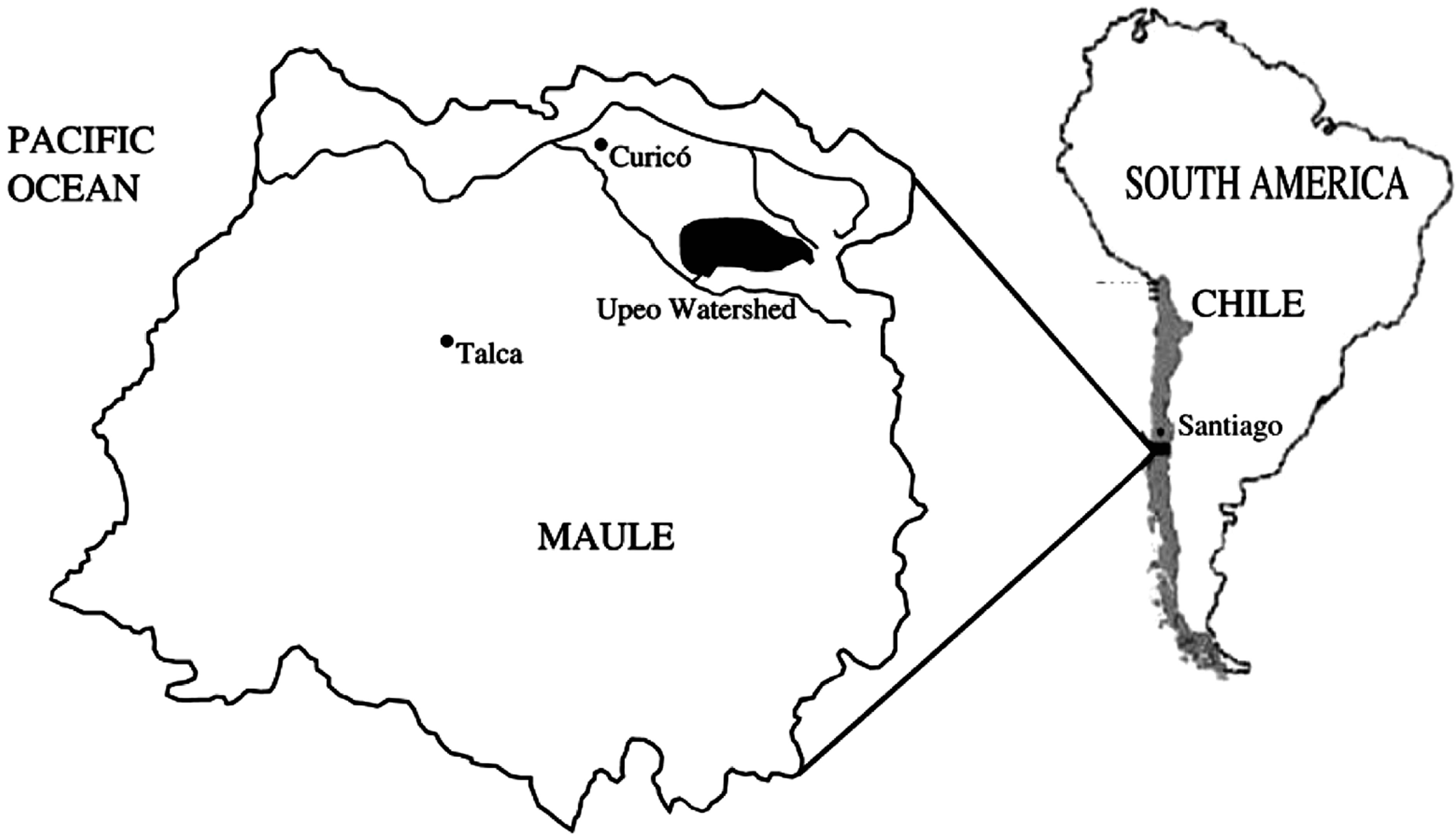
Figure 1. The lacation of the Upeo watershed within the region of Maule.
widely used method used to date developed by Linsley et al. [9] with the approach we are proposing here (henceforth referred to as the original and modified approaches respectively). Using discharge data for a small watershed located in the Andes mountain range of central Chile we compared the two onset point definitions using various baseflow recession equations in order to determine whether the modified approach more accurately models observed baseflow behavior.
Site Description
The Upeo is a snow-fed creek that originates in the Andes mountain range of central Chile, running for 126 km before discharging into the Lontué River en route to the Pacific Ocean [10]. Its watershed covers a surface area of 2510 km2 and receives close to 1800 mm of precipitation annually. Annual average flows are estimated at 78.9 m3·s−1 [11].
The Chilean government agency in charge of managing the country’s water resources, the Dirección General de Aguas (DGA), manages a gauging stationat the confluence of the Upeo and the Lontué River (35˚10'23"S lat; 71˚05'28"W long). Using limnograph and discharge curve data from the Upeo Station, storm hydrographs and baseflow recession curves were created for 27 storm events from the period of 1982-1995. Storm events used in this analysis were chosen based on having the most continuous and extensive data available for the falling limb of the storm hydrographs.
2. Methods
2.1. Graphical Definition of Baseflow Recession Onset
A storm hydrograph, a graphical representation of the relationship between channel flow versus time during a storm event, is characterized by a rising limb, a peak flow, a falling limb, and a baseflow recession curve [12]. The response of the storm hydrograph is affected by a combination of watershed and climatic characteristics, which include hydrologic losses and surface runoff characteristics, among other variables [3].
The general shape of a storm hydrograph is shown in Figure 2. The most commonly used protocol to separate hydrographs was developed by Linsley et al. [9] and consists of drawing an imaginary line from point A that continues the trajectory of the baseflow recession curve prior to the onset of the storm until peak flow (point B) has been reached. After peak flow is reached, subsurface (seepage) flows are considered to be contributing to channel flow and a second line is drawn to point C, from which point on channel flow is solely comprised of groundwater contributions (baseflow recession).
Baseflow recession onset is identified using data from the falling limb of the storm hydrograph, which is plotted on a logarithmic graph of flow versus time where it presents as a linear graphic distribution with three inflection points. The use of the second inflection point (Point C in Figure 3) to define baseflow recession onset corresponds to the original approach developed by Linsley et al. [9]; the modified approach being proposed here redefines baseflow onset as the third inflection point on the same graph (Point D). Other hydrograph separation methodologies, such as those proposed by Bedient and Hubert [3] and Viessman and Lewis [5], offer more rough approximations of baseflow recession behavior but were not considered appropriate for the type of analysis used in this study.
2.2. Baseflow Recession Equations
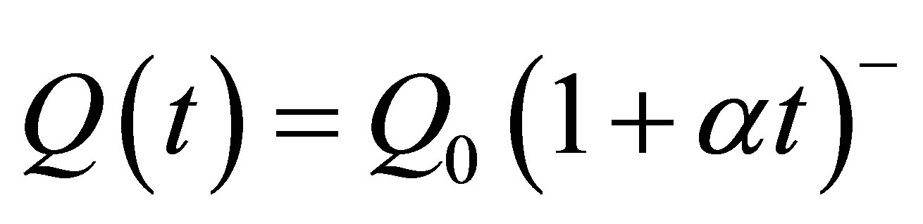
Baseflow recession equations are derived from the base model [3]:
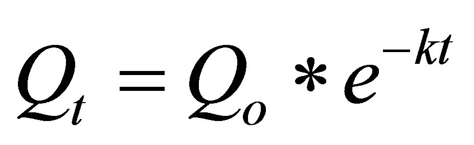 (1)
(1)
where Q0 represents baseflow volume in m3·s−1 at time t0, Qt is baseflow volume in m3·s−1 at time t, e is the Neper
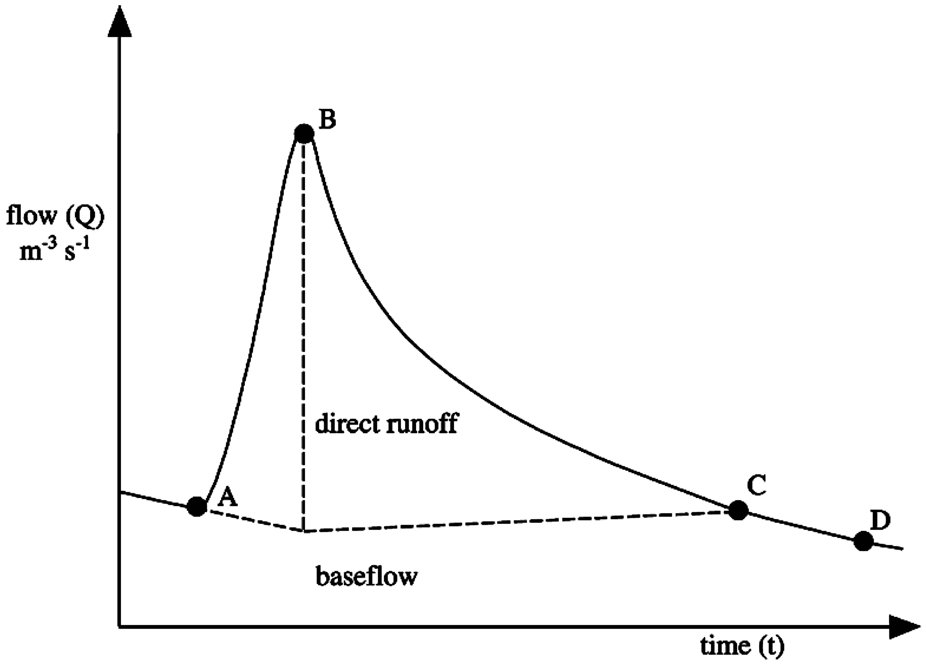
Figure 2. General storm hydrograph form and characteristics proposed by Linsley et al. [9] Adapted from Chow et al. [13].
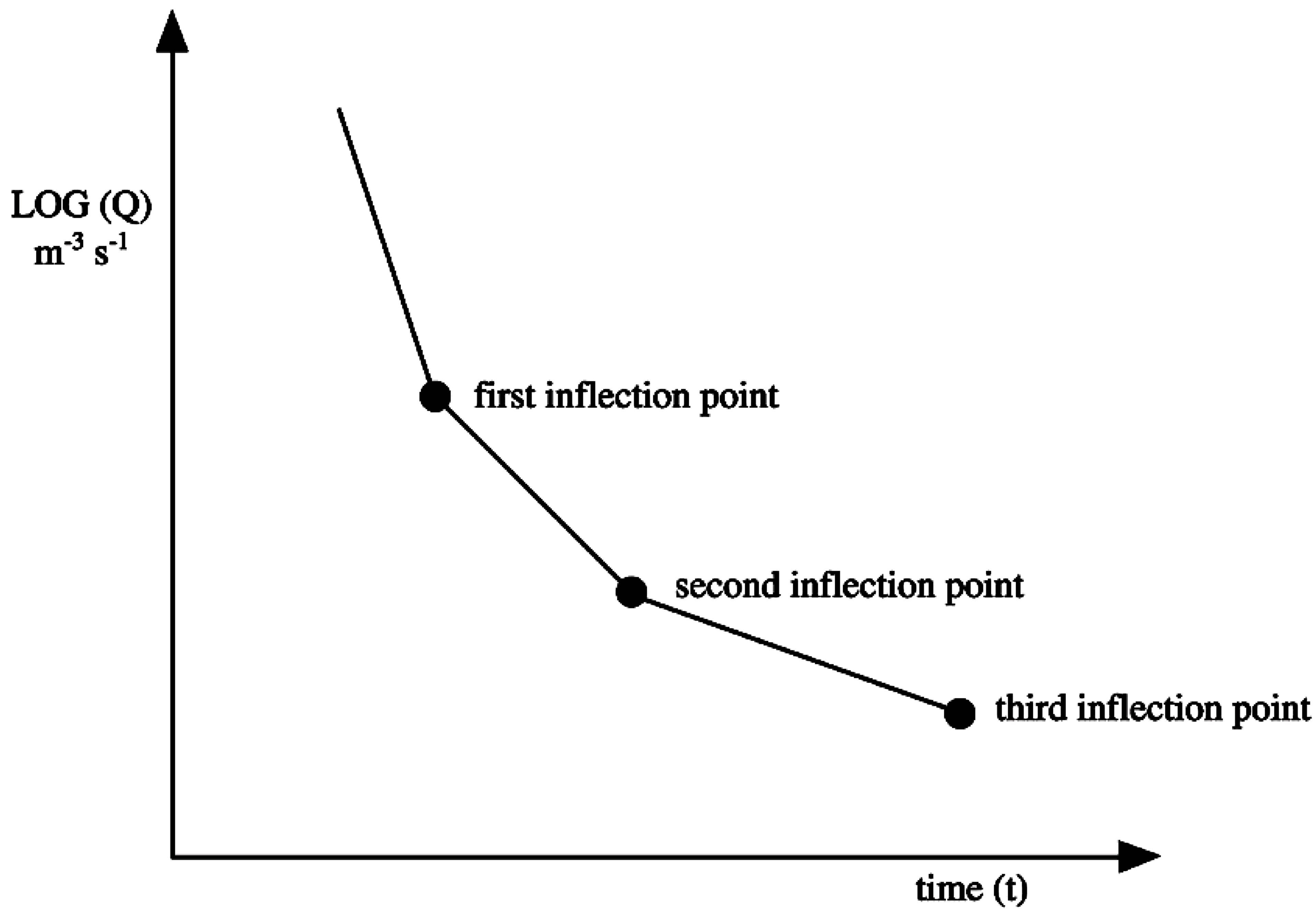
Figure 3. An example of the falling limb of a storm hydrograph and its inflection points.
constant, and k is the recession coefficient. The original and modified approaches were compared by defining time t0 as either the second (Point C) or third (Point D) inflection point.
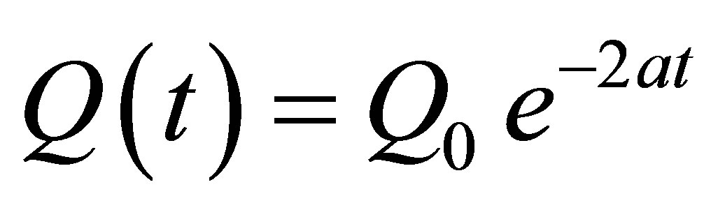
The equations used in this comparison were required to accurately reflect the behavior of flow as decreasing as a function of time at the onset of baseflow recession (Pizarro, 1993), or in other words satisfy the condition q/dt < 0 at t0. Widely used models by authors such as Remenieras [14], Singh [15], and Maidment [12] were considered. However, the following three models were selected for use based on their statistical accuracy with observed data (defined as higher R2 and lower SEE values):
 (2)
(2)
 (3)
(3)
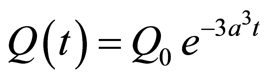 (4)
(4)
Equation parameters are identical to Equation (1) above, with the exception of alpha (α), which replaces k as the recession coefficient.
In order to determine if an increase in elapsed time from point t0 would help the models to better reflect the observed data, the following five time intervals were chosen to adjust the model parameter of time t: 10, 15, 20, 24, and 48 hours, all of which were used previously with satisfactory results.
Next, the results for the three equations using the original and modified approaches were calibrated and validated in comparison with the observed data [15]. We used the coefficient of determination (R2) and the standard error of estimation (SEE) to validate results along with the following statistical tests: the Mann-Whitney U test, whose central objective is to determine whether or not independent samples come from the same population [16], and the Bland-Altman test, which quantifies the difference between the observed and modeled data [17]. All statistical analyses were evaluated using a significance level α = 0.05.
3. Results and Discussion
The data for the 27 storm events used in this study along with their corresponding Q0 values for the original and modified approaches are shown in Table 1. The high variability shown in the data made it difficult to develop a precise equation specific to the data.
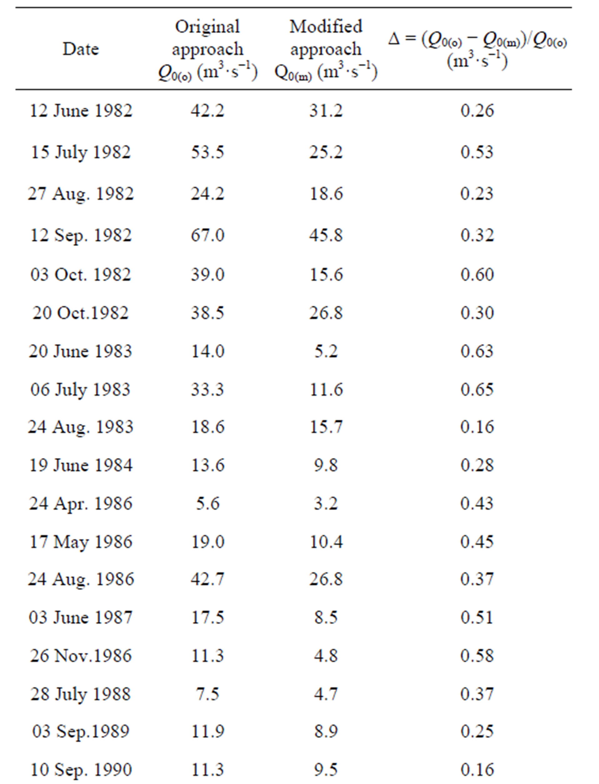
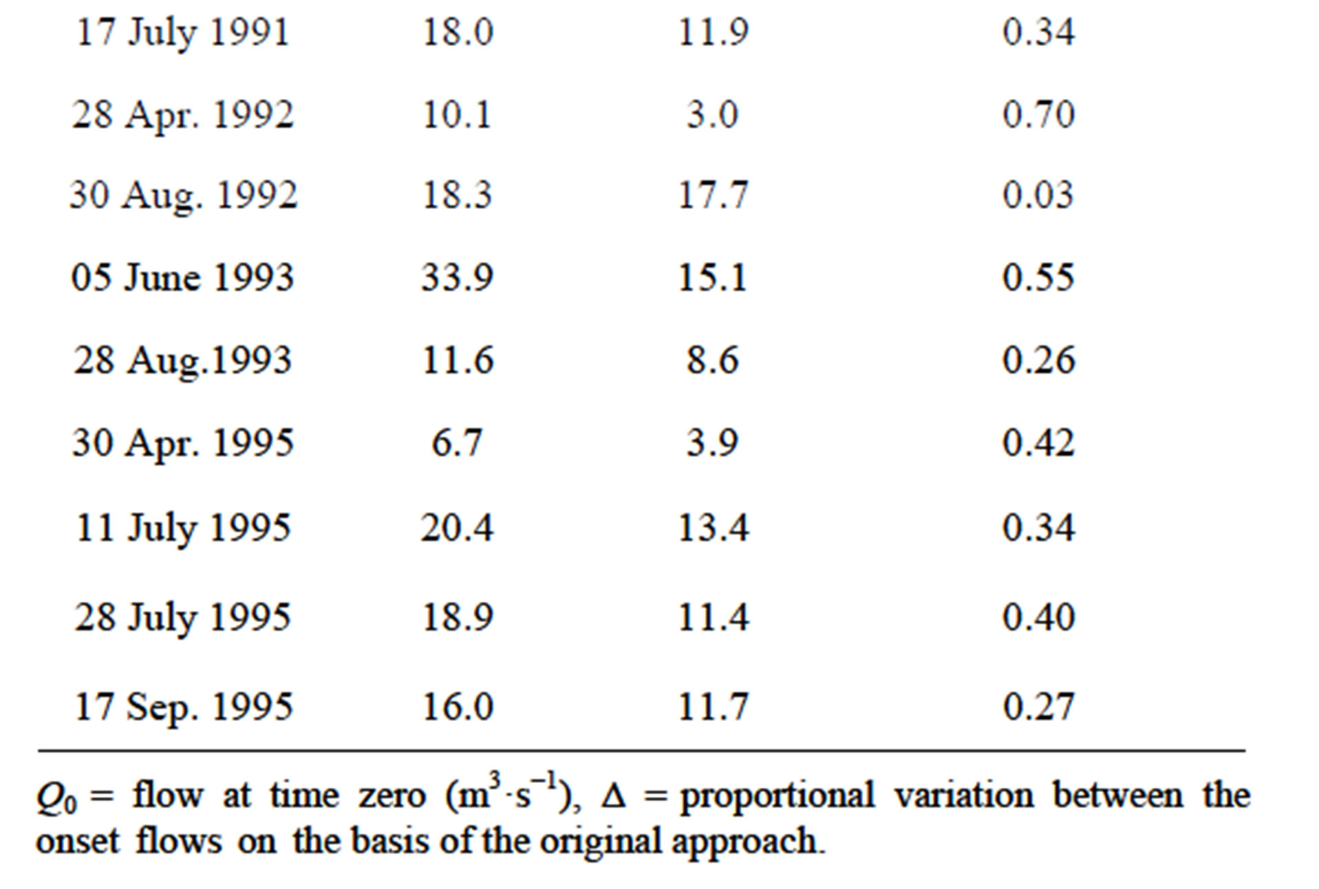
Table 1. Dates and onset flows using the original and modified approaches for the 27 studied flood events.
For the original and modified approaches, Equations (3) and (4) both overestimated whereas quadratic Equation (2) slightly underestimated observed flow. For all three models values for the recession coefficient α averaged higher for the original approach than the modified (Tables 2(a) and (b)), which was to be expected as the displacement of Q0 from the second to third inflection point significantly altered the slope of the curve.
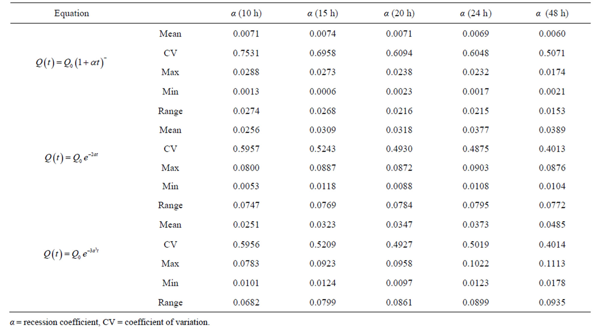 (a)
(a)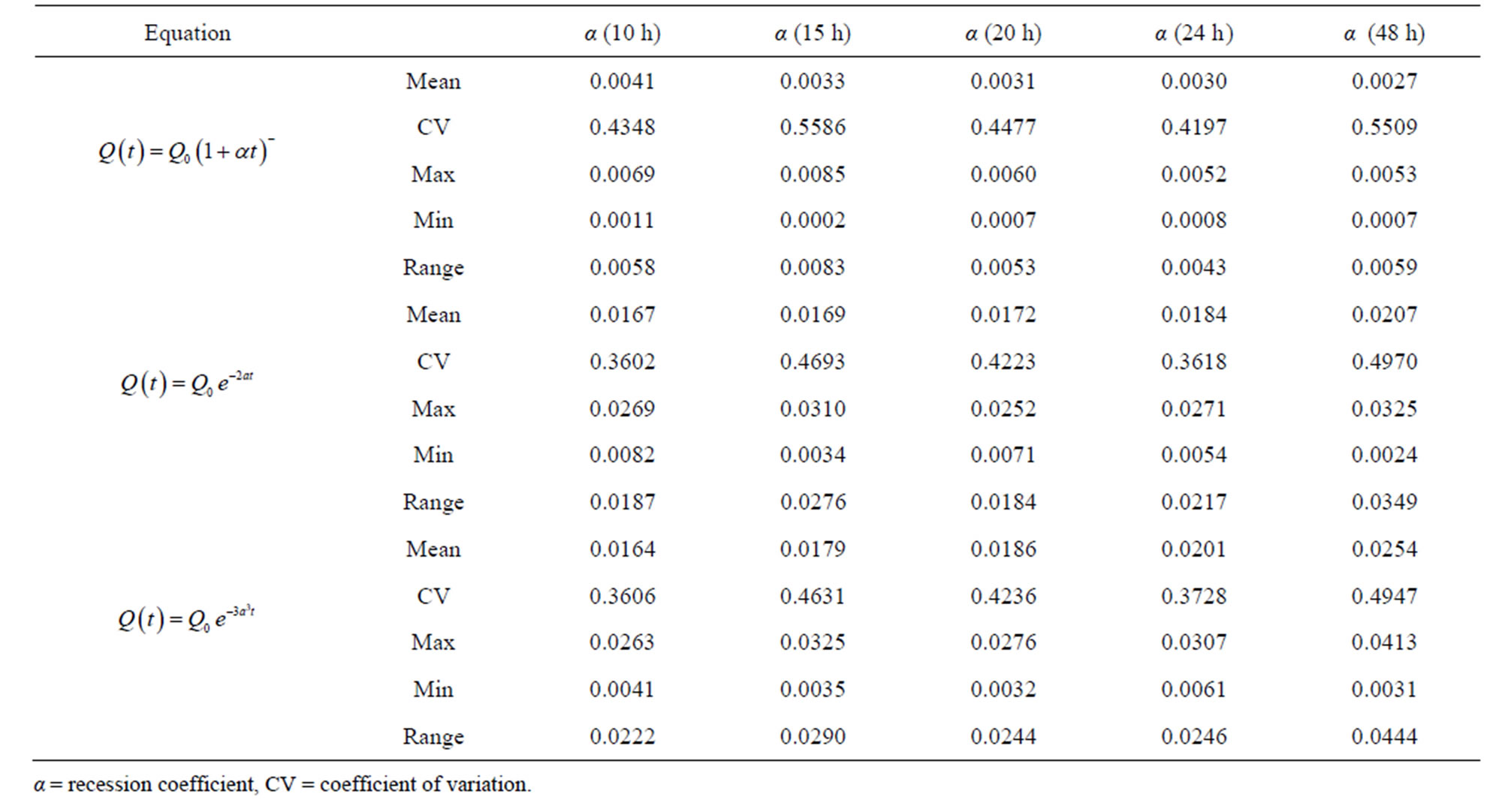 (b)
(b)
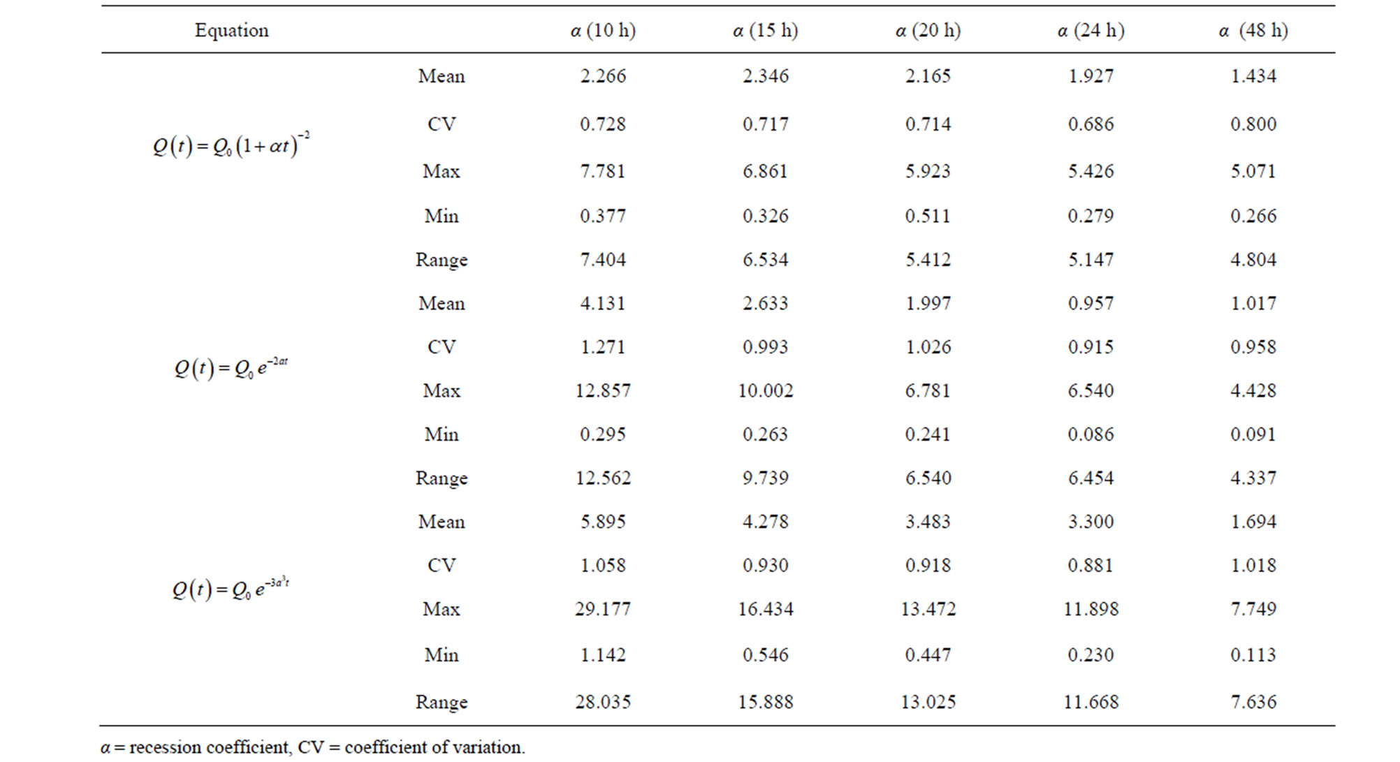
Table 2. (a) Recession coefficient values α for the equations using the original approach; (b) Recession coefficient α values for the equations using the modified approach.
Coefficient of determination values (R2) were generally low for both approaches (Tables 3(a) and (b)), but were relatively higher for the original approach. However, SEE tended to decrease with an increase in elapsed time for the original approach (Tables 4(a) and (b)), reaching a minimum for Equations (2) and (4) at hour 48;
 (a)
(a)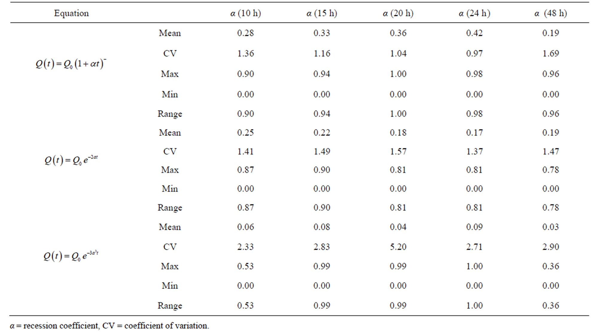 (b)
(b)
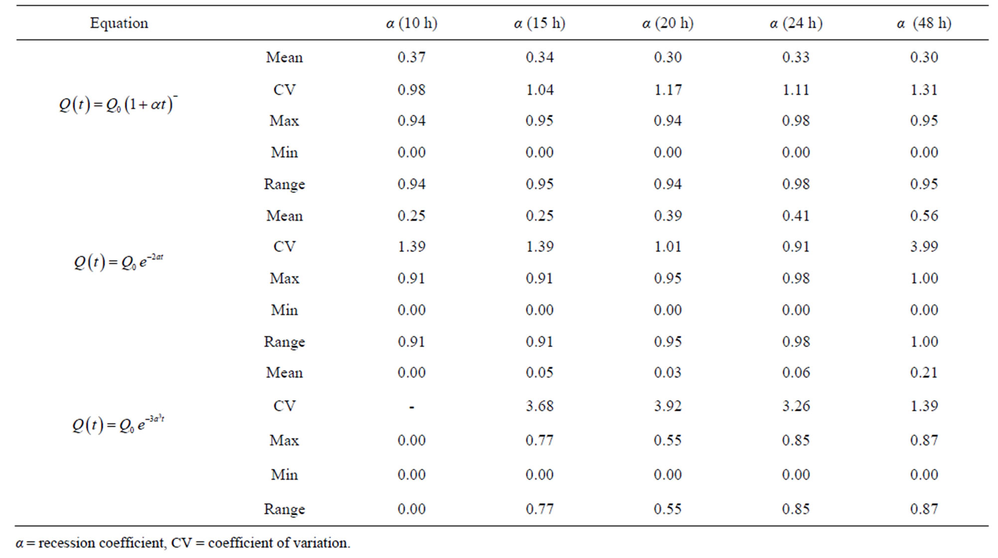
Table 3. (a) Coefficient of determination R2 values for the equations using the original approach; (b) Coefficient of determination R2 values for the equations using the modified approach.
 (a)
(a)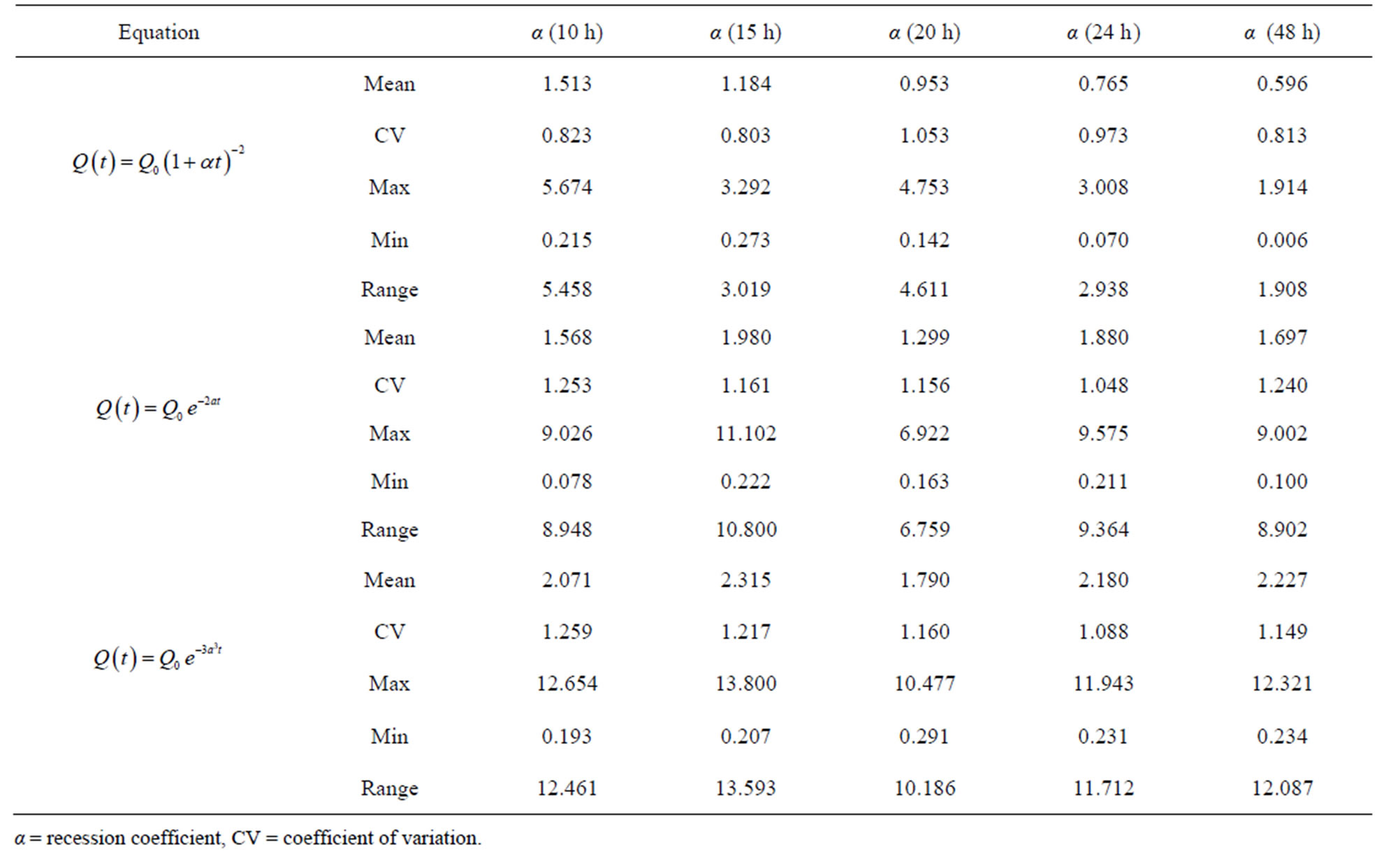 (b)
(b)
Table 4. (a) SEE values for the equations using the original approach; (b) SEE values for the equations using the modified approach.
α = recession coefficient, CV = coefficient of variation.
and for Equation (3) at hour 24. This decrease in accuracy with an increase in elapsed time is in direct disagreement with the R2 analysis, which could be explained by the fact that R2 is independent of SEE and only quantifies the variability in the data.
On the other hand, only Equation (2) saw a decrease in SEE values for an increase in elapsed time using the modified approach. Regardless, all three equations obtained smaller SEE values for the modified approach than the original. This, along with the corresponding R2 values, clearly suggests that the modified approach better adjusts to observed data.
To further the statistical analysis average observed values were compared by obtaining the quotients between SEE and the observed flows for the 27 selected storm events for the respective equation, approach, and time interval. A recession coefficient α value of 48 hours produced the best results for the original approach, as shown in Tables 5(a) and (b). Only Equation (2) showed an increase in accuracy with a corresponding increase in the amount of elapsed time for the modified approach.
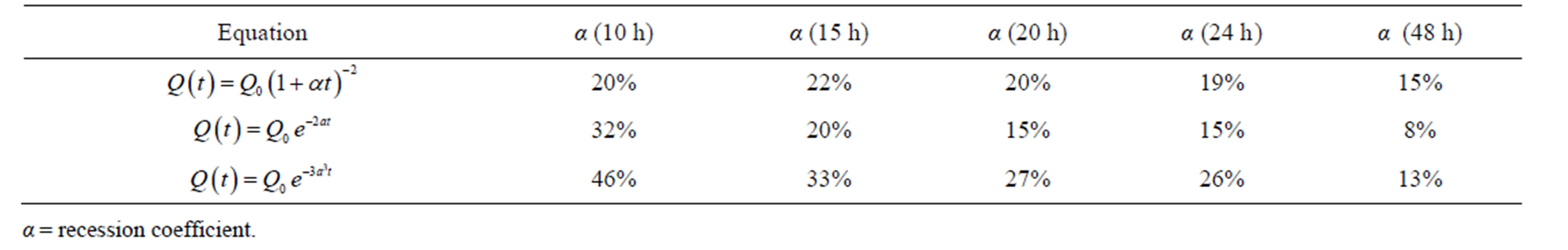
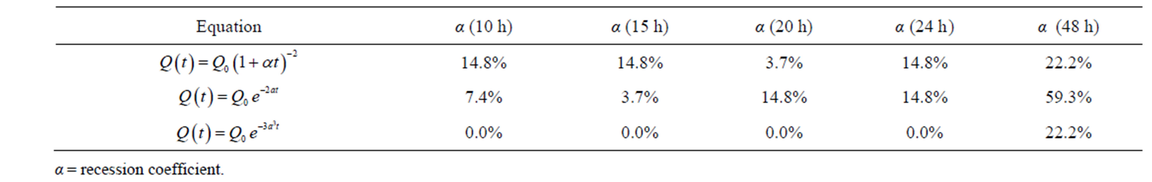
Results from the Mann-Whitney U test are shown in Tables 6(a) and (b), where the percentage of accepted tests for the three equations and five time intervals are tabulated for ease of interpretation. According to the analysis, Equation (3) had the highest number of accepted tests for the original approach, whereas Equation (2) was superior for the modified approach. The modified approach showed the highest acceptance rate for all time intervals and equations analyzed.
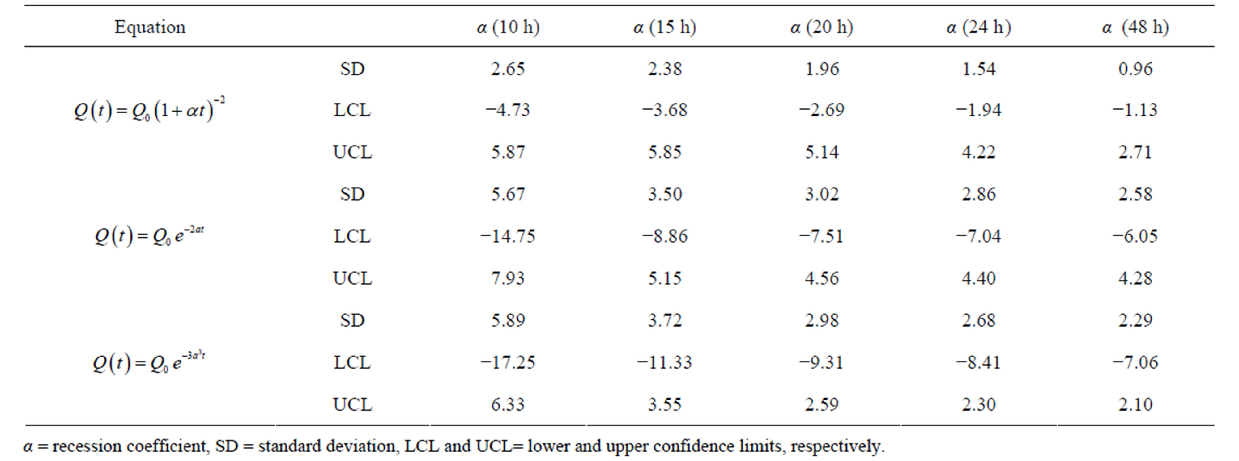
Finally, the results for a comparison between observed and modeled data using the Bland-Altman test are shown in Tables 7(a) and (b). Results indicate that the standard deviations of mean difference are significantly lower for
 (a)
(a)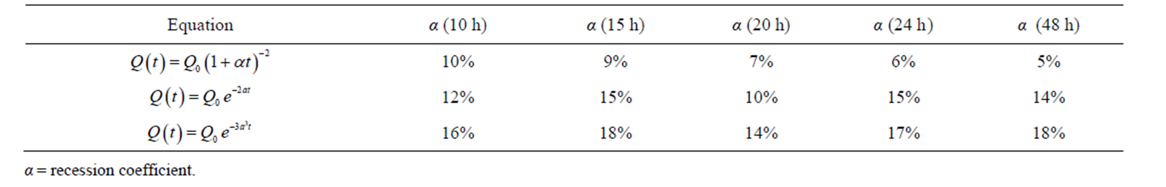 (b)
(b)
Table 5. (a) Quotients between SEE and average observed flows for the equations using the original approach; (b) Quotients between SEE and average observed flows for the equations using the modified approach.
 (a)
(a)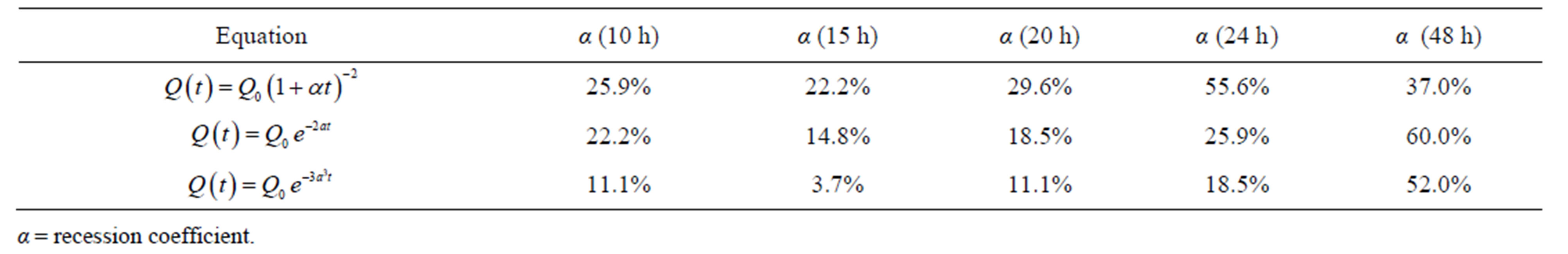 (b)
(b)
Table 6. (a) Approval percentages for the Mann-Whitney U test for the equations using the original approach; (b) Approval percentages for the Mann-Whitney U test for the equations using the modified approach.
 (a)
(a)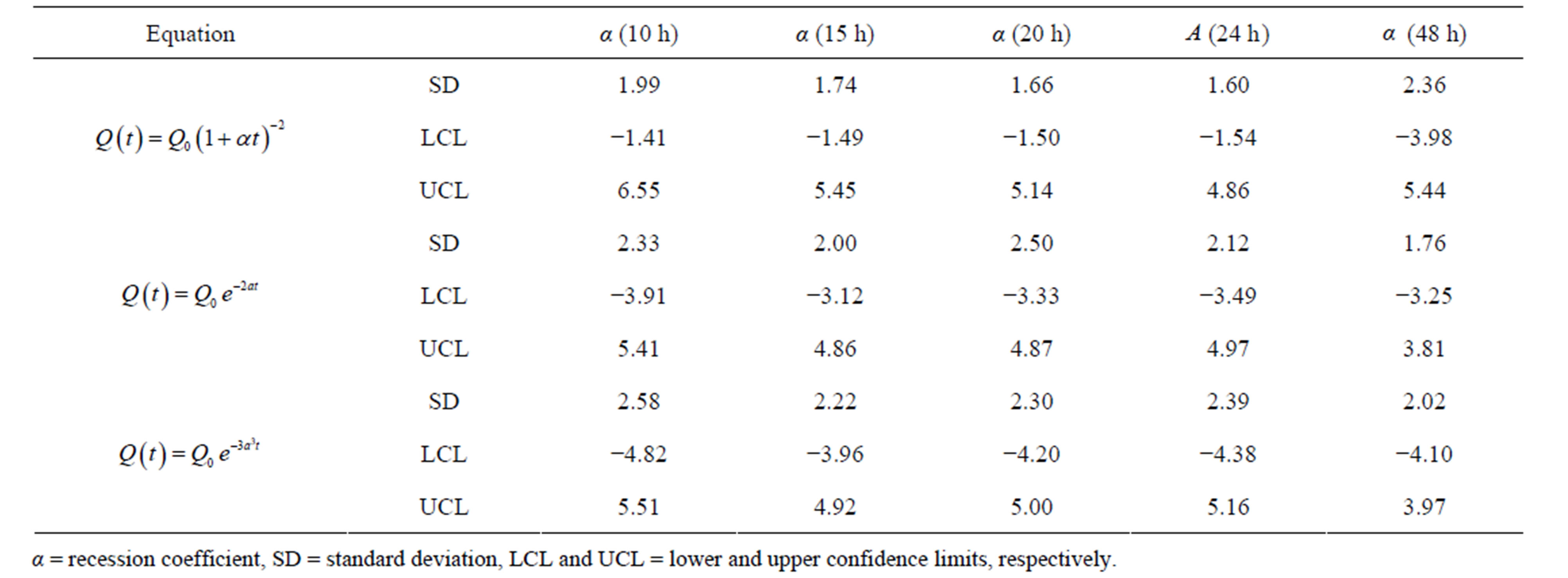 (b)
(b)
Table 7. (a) Results for the Bland-Altman test applied to the equations using the original approach; (b) Results for the Bland-Altman test applied to the equations using the modified approach.
the modified approach, which is further supported by the confidence interval analysis. Similarly, data dispersion around the mean values was more uniform for the modified approach.
4. Conclusions and Recommendations
On the basis of the completed statistical analyses for all three selected equations, in particular the results of the Mann-Whitney U test, we conclude that the modified approach more accurately predicts baseflow recession behavior; or, that model accuracy is improved by defining the onset of baseflow recession as the third inflection point of the logarithmic graph of the falling limb of the storm hydrograph. Results of this study question the feasibility of continuing to use the current hydrograph separation procedure proposed in 1949 by Linsley et al. [9]. We strongly recommend considering this new modified approach for future studies.
Of the three selected and analyzed equations, the quadratic model Equation (2) offered the best modeling results. However, the authors recommend continuing to test other equations to improve even more the estimation of baseflow recession, as well as the use of more statistical parameters besides the coefficient of determination R2.
REFERENCES
- M. Manga, “Origin of Post Seismic Stream Flow Changes Inferred from Baseflow and Magnitude-Distance Relations,” Geophysical Research Letters, Vol. 28, No. 10, 2001, pp. 2133-2136. http://dx.doi.org/10.1029/2000GL012481
- V. Ponce, “Engineering Hydrology, Principles and Practices,” Prentice Hall College Division, New Jersey, 1989.
- P. Bedient and W. Huber, “Hydrology and Floodplain Analysis,” 3rd Edition, Prentice Hall, Englewood Cliffs, 2002.
- R. Linsley and M. Kohler, “Hydrology for Engineers,” 2nd Edition, McGraw-Hill, New York, 1975.
- W. Viessman and G. Lewis, “Introduction to Hydrology,” 5th Edition, Prentice Hall, Engelwood Cliffs, 2003.
- G. N. Martin, “Characterization of Simple Exponential Baseflow Recessions,” New Zealand Journal of Hydrology, Vol. 12, No. 1, 1973, pp. 57-62.
- T. Chapman, “A Comparison of Algorithms for Stream Flow Recession and Baseflow Separation,” Hydrological Processes, Vol. 13, No. 5, 1999, pp. 701-714. http://dx.doi.org/10.1002/(SICI)1099-1085(19990415)13:5<701::AID-HYP774>3.0.CO;2-2
- R. Vogel and C. Kroll, “Estimation of Baseflow Recession Constants,” Water Resources Management (Netherlands), Vol. 10, No. 4, 1996, pp. 303-320. http://dx.doi.org/10.1007/BF00508898
- R. Linsley, M. Kohler and J. Paulhus, “Applied Hydrology,” McGraw-Hill, New York, 1949.
- H. Niemeyer and P. Cereceda, “Hidrografía. Geografía de Chile. Tomo VIII,” Instituto Geográfico Militar de Chile, Santiago, 1983.
- Dirección General de Aguas (DGA), “Estudio del Mapa Hidrogeológico Nacional,” 1986.
- D. Maidment, “Handbook of Hydrology,” McGraw-Hill, New York, 1993.
- V. Chow, D. Maidment and L. W. Mays, “Applied Hydrology,” McGraw-Hill, New York, 1949.
- G. Remenieras, “Tratado de Hidrología Aplicada. Primera Edición Española,” Técnicos Asociados S.A. Barcelona, Spain, 1971.
- V. Singh, “Hydrologic Systems: Rainfall-Runoff Modeling,” Prentice Hall, Englewood Cliffs, 1988.
- R. Mason and D. Lind, “Statistical Techniques in Business and Economics,” 8th Edition, University of Toledo, Ohio, 1998.
- J. Bland and D. Altman, “Measuring Agreement in Method Comparison Studies,” Statistical Methods in Medical Research, Vol. 8, No. 2, 1999, pp. 135-160. http://dx.doi.org/10.1191/096228099673819272