Theoretical Economics Letters
Vol.2 No.5(2012), Article ID:25804,5 pages DOI:10.4236/tel.2012.25087
Equilibrium Dynamics in the Neoclassical Growth Model with Habit Formation and Elastic Labor Supply
Department of Applied Economics II, University of A Coruña, Galicia, Spain
Email: mago@udc.es
Received September 15, 2012; revised October 16, 2012; accepted November 18, 2012
Keywords: Economic Growth; Habit Formation; Equilibrium Dynamics
ABSTRACT
This note analyzes the equilibrium dynamics in the neoclassical growth model with habit-forming preferences and elastic labor supply. Habits enter into utility in a multiplicative way. The specification of the habit formation process comprises the particular cases of internal and external habits. Existence, uniqueness and saddle-path stability of the steady state are proved analytically.
1. Introduction
This note analyzes the equilibrium dynamics in the neoclassical growth model with habit formation and elastic labor supply. In our model utility is additively separable and CRRA in adjusted consumption and leisure, and habits enter utility in a multiplicative way. These are specifications commonly used in the literature. Specifically, we demonstrate analytically that the steady state is unique and (locally) saddle-path stable, so that the equilibrium is (locally) uniquely determined.
Habit-forming preferences have been widely incorporated to dynamic macroeconomic models. The reason is that they help to explain some empirical facts difficult to accommodate with standard time-separable preferences as, e.g., the equity premium puzzle (e.g., [1,2]), the savings-growth nexus (e.g., [3]) or the effects of monetary policy (e.g., [4]). In habit-formation models individual’s utility depends on her current consumption and also on how it compares to a reference level of consumption— the habits stock. The literature distinguishes between internal habits (IH), which are formed from individual’s own past consumption (e.g., [2,4]), and external habits (EH), which are formed from average economy-wide past consumption (e.g. [1,5]). Hence, we consider a specification of the habit formation process which comprises the particular cases of internal and external habits.
Previous work has analyzed the equilibrium dynamics of growth models with habit formation, mainly in AKtype growth models (e.g. [6-10]). However, in all these works labor supply is assumed to be inelastically provided. A notable exception is [11], which considers a growth model with elastic labor supply. Given the complexity of the system that drives the dynamics of the economy, saddle-point stability of the steady state in this kind of models is often taken as guaranteed and sometimes supported by numerical simulations (e.g. [9,11])1. The present paper demonstrates that economies, as described above, do in fact generally have saddlepoint stable steady states. Therefore, this paper is also related to previous works that study analytically the stability properties of equilibrium in growth models (e.g. [12,13]), or that intend to provide solid mathematical foundations to growth models with habit formation (e.g., [8,14,15]).
The remaining of the paper is organized as follows. Section 2 presents the model. Section 3 analyzes the equilibrium dynamics. Section 4 concludes.
2. Setup of the Model
Consider an economy populated by N identical infinitely-lived representative agents that grows at the exogenous rate . The intertemporal utility derived by the agent is
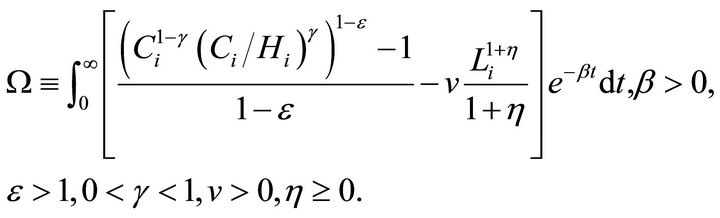 (1)
(1)
where Ci and Hi are agent’s i consumption and reference consumption level (habits stock), respectively, Li is agent’s i work time, g reflects the importance of habits in utility, b is the rate of time preference, h denotes the inverse of the labor supply elasticity, and 1/e is the intertemporal elasticity of substitution of consumption in the time-separable case . The assumption that
  is taken from [8,14], which show that otherwise the optimization problem might not be well-defined in a similar model with inelastic labor supply.
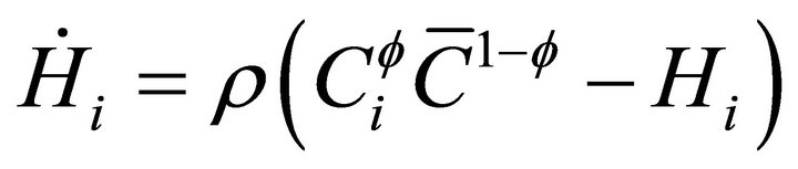
Following [9], the reference consumption level is formed as an exponentially declining average of past consumption according to
 (2)
(2)
where 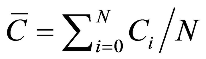 denotes the economy-wide average consumption. Setting f = 1 corresponds to the internal habit formation case, in which the reference stock is formed as an exponentially declining average of own past consumption. Setting f = 0 corresponds to the external habit formation case, in which the reference stock is formed as an exponentially declining average of economy-wide average past consumption. The case 0 < f < 1 corresponds to an intermediate case, in which the reference stock is formed as an exponentially declining average of own and average past consumption. The rate of adjustment of the reference stock is then
 (3)
(3)
Individual output, Yi, is determined by the CobbDouglas technology
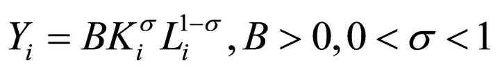 , (4)
, (4)
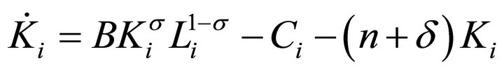
where Ki is the individual’s capital stock. The agent’s budget constraint is
 (5)
(5)
where d is the rate of depreciation of capital.
3. The Equilibrium
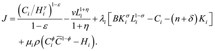
The agent chooses Ci, Li, Ki, and Hi to maximize individual’s intertemporal utility (1) subject to her budget constraint (5) and the constraint on the accumulation of the habits stock (3). Let J be the current value Hamiltonian of the agent’s optimization problem,
The first-order conditions for an interior optimum are
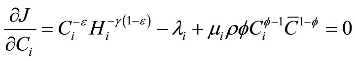 (6a)
(6a)
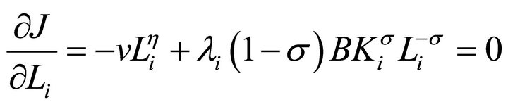 (6b)
(6b)
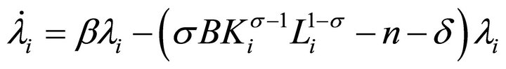 (6c)
(6c)
 (6d)
(6d)
plus the transversality condition
 (6e)
(6e)
We focus on a symmetric equilibrium in which, with all agents being identical,  . Hence, (6a) yields
 . (7)
. (7)
Defining , from (7) we get
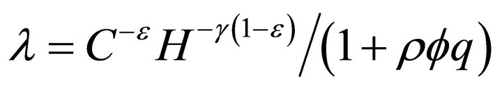 , (8a)
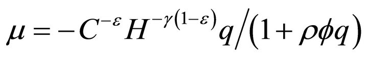 (8b)
(8b)
From (6b) and (8a), we find the following expression of the work time L as a function of K, C, H and q:
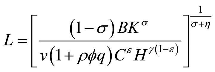 (9)
(9)
Differentiating (7) with respect to time, we get
 . (10)
From (7) and (6b), we obtain
 (11)
(11)
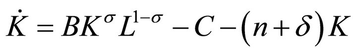
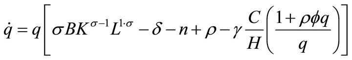
The system that drives the dynamics of the economy is
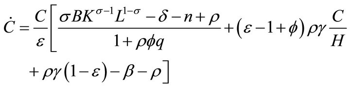 (12a)
(12a)
 (12b)
(12b)
 (12c)
(12c)
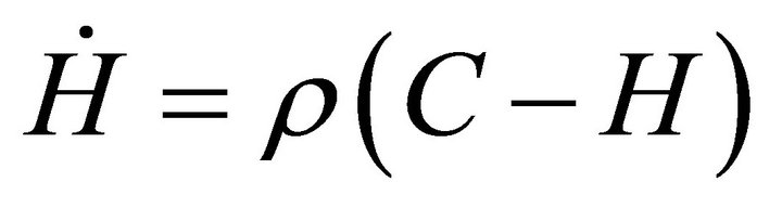 (12d)
(12d)
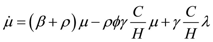
where L is given by (9). Equation (12d) is obtained from (3), using that . Equation (12a) is obtained by substituting for
  from (12d),
  from (6c) and
  from (11) into (10), and using (8). Equation (12b) is the budget constraint (5). Equation (12c) is obtained by substituting for
  from (6c) and
  from (11) into
 .
.
Now, we focus on an interior steady state. An overline will denote the steady-state value of a variable. The following proposition states the existence and uniqueness of a steady state.
Proposition 1. The economy has a unique steady state
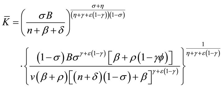 (13a)
(13a)
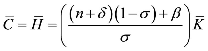 (13b)
(13b)
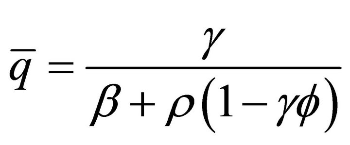 (13c)
(13c)
and the steady-state value of the work time is
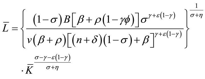 (13d)
(13d)
Proof. Let . Imposing
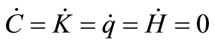 , the steady state of (12) is the solution of the system
 (14)
(14)
 (15)
(15)
 (16)
(16)
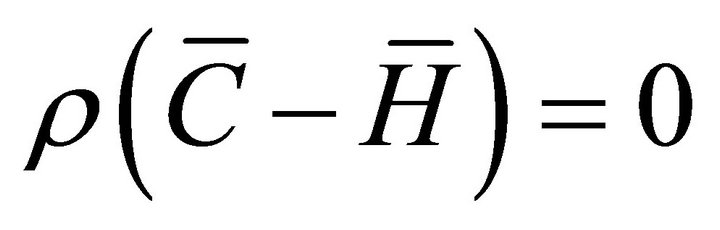 (17)
(17)
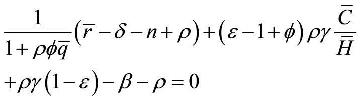
Equation (17) entails that , which substituted into (14) yields
 (18)
(18)
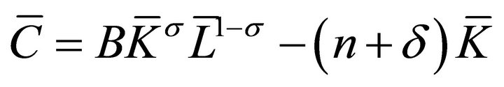
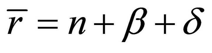
From (16) and (18), we obtain (13c). Now, from (18) we get
 (19)
(19)
From (19) and , we have that
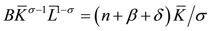 , which substituted into (15) yields (13b). Substituting
  and
and  for (13b) into (9) we get (13d). Substituting
  for (13d) into
 , using (19), we get (13a) after simplifycation. The transversality condition (6e) can be easily shown to be equivalent to
 . ■
. ■
The following Lemma will be used to study the stability of the steady state.
Lemma 1. Let the characteristic equation for a matrix B of order 4 ´ 4 be
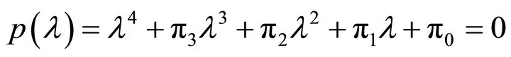 .
.
If , the matrix B features two (stable) roots with negative real parts.
Proof. The number of roots of the characteristic equation with negative real parts (stable roots) is equal to the number of roots of the polynomial 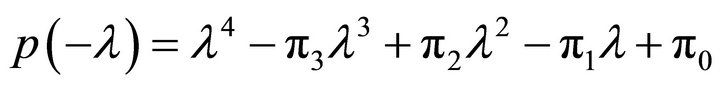 with positive real parts. Using the Routh-Hurwitz theorem (e.g., [16]), the number of stable roots is then equal to the number of variations of sign in the scheme
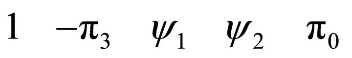
where 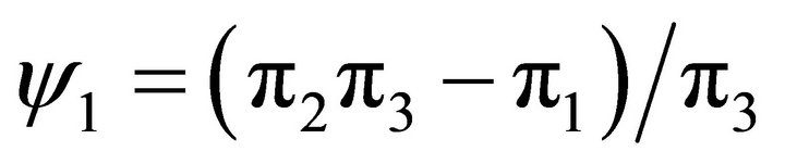 and
and  . If
. If  then
then , and so, we have the scheme
Hence, there are two variations in sign. If  we have the configuration
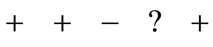
where a question mark represents an unknown sign, which could be even zero. Irrespective of the unknown sign (even if it is zero), there are two variations in sign. If , we substitute
  for a positive constant e than tends to zero, and we obtain the following configuration
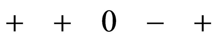
Since the sign of the entry to the left of the zero is different to that to the right of it, this indicates a change of sign, and so, there are two variations in sign. Hence, in any case there are two variations in sign, and so, B has two (stable) roots with negative real parts. ■
The following proposition establishes the saddle-path stability of the steady state.
Proposition 2. The steady state of the economy described by (13a)-(13c) is locally saddle-path stable.
Proof. Linearizing (12) around its steady state (13) we obtain
 (20)
(20)
where
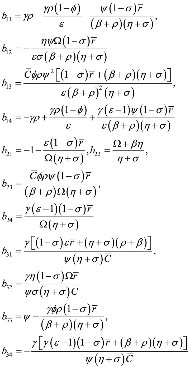
with ,
, 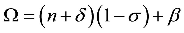 , and
, and 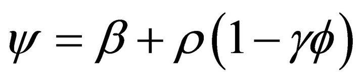 .
.
The characteristic equation for the matrix B is

where p3 is the opposite of the trace of B,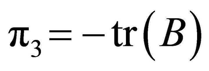 ; p2 is the sum of all the leading principal minors of order 2 of B; p1 is the opposite of the sum of all the leading principal minors of order 3 of B, and p0 is the determinant of B,
 . It can be proved by direct computation that
Using Lemma 1, the matrix B has two stable roots. Since the system (12) features two predetermined variables, K and H, the number of stable roots is equal to the number of predetermined variables. Hence, the steady state  is locally saddle-path stable. ■
In accordance with the results reported in [9] for a similar model with inelastic labor supply, numerical experimentation shows that the stable roots may also be real or complex when labor supply is elastically supplied. For example, the parameterization B = 1, s = 0.4, b = 0.04, n = 0.01, d = 0.04, e = 1.5, g = 0.3, r = 0.1, v = 4, h = 0.8, f = 1 yields the (complex) stable roots –0.08597 ± 0.01709i. If the speed of adjustment is reduced from r = 0.1 to r = 0.02, the (real) stable roots are –0.08942 and –0.01812. Hence, the equilibrium path could converge to the steady state through damped oscillations.
4. Conclusions
This paper has analyzed the equilibrium dynamics of the neoclassical growth model with multiplicative habits and elastic labor supply. The specification of habit formation comprises the particular cases of internal and external habits. Uniqueness and saddle-path stability of the steady state is proved analytically. The stability analysis shows that the transitional dynamics of the model is represented by a two-dimensional stable saddle-path. This provides a much richer dynamics for the transition paths relative to the standard neoclassical growth model without habits (e.g., [17]) or the AK endogenous growth model with habit formation (e.g., [6]) that feature a single stable root and a one-dimensional stable saddle-path.
In this paper we have assumed that leisure and adjusted consumption are additively separable in utility, and that habits enter utility in a multiplicative way. Interesting extensions would be to analyze whether the saddle-point stability result is robust with respect to a non-separable specification of adjusted-consumption and leisure, and with respect to habits entering utility in an subtractive way (e.g., [2]) or even in a more general way (e.g., [18,19]). These issues will be the subject of future research.
5. Acknowledgements
The author wishes to thank an anonymous referee for useful comments. Financial support from the Spanish Ministry of Science and Innovation through Grant ECO2011- 25490 is gratefully acknowledged.
REFERENCES
- A. Abel, “Asset Prices under Habit Formation and Catching up with the Joneses,” American Economic Review, Vol. 80, No. 2, 1990, pp. 38-42.
- G. M. Constantinides, “Habit Formation: A Resolution of the Equity Premium Puzzle,” Journal of Political Economy, Vol. 98, No. 3, 1990, pp. 519-543. doi:10.1086/261693
- C. D. Carroll, J. Overland and D. N. Weil, “Saving, Growth and Habit Formation,” American Economic Review, Vol. 90, No. 3, 2000, pp. 341-355. doi:10.1257/aer.90.3.341
- J. C. Fuhrer, “Habit Formation in Consumption and Its Implications for Monetary Policy Models,” American Economic Review, Vol. 90, No. 3, 2000, pp. 367-390. doi:10.1257/aer.90.3.367
- J. Campbell and J. Cochrane, “By Force of Habit: A Consumption-Based Explanation of Aggregate Stock Market Behavior,” Journal of Political Economy, Vol. 107, No. 2, 1999, pp. 205-251. doi:10.1086/250059
- C. D. Carroll, J. Overland and D. N. Weil, “Comparison Utility in a Growth Model,” Journal of Economic Growth, Vol. 2, No. 4, 1997, pp. 339-367. doi:10.1023/A:1009740920294
- M. A. Gómez, “Optimal Consumption Taxation in a Model of Endogenous Growth with External Habit Formation,” Economics Letters, Vol. 93, No. 3, 2006, pp. 427-435. doi:10.1016/j.econlet.2006.06.017
- J. Alonso-Carrera, J. Caballe and X. Raurich, “Growth, Habit Formation, and Catching-Up with the Joneses,” European Economic Review, Vol. 49, No. 6, 2005, pp. 1665-1691. doi:10.1016/j.euroecorev.2004.03.005
- F. Alvarez-Cuadrado, G. Monteiro and S. J. Turnovsky, “Habit Formation, Catching-Up with the Joneses, and Economic Growth,” Journal of Economic Growth, Vol. 9, No. 1, 2004, pp. 47-80. doi:10.1023/B:JOEG.0000023016.26449.eb
- M. A. Gómez, “Equilibrium Efficiency in the Ramsey Model with Habit Formation,” Studies in Nonlinear Dynamics & Econometrics, Vol. 11, No. 2, 2007, p. 2.
- S. J. Turnovsky and G. Monteiro, “Consumption Externalities, Production Externalities, and Efficient Capital Accumulation under Time Non-Separable Preferences,” European Economic Review, Vol. 51, No. 2, 2007, pp. 479-504. doi:10.1016/j.euroecorev.2005.12.001
- L. G. Arnold, “The Dynamics of the Jones R & D Growth Model,” Review of Economic Dynamics, Vol. 9, No. 1, 2006, pp. 143-152. doi:10.1016/j.red.2005.09.001
- D. Mondal, “Stability Analysis of the Grossman-Helpman Model of Endogenous Product Cycles,” Journal of Macroeconomics, Vol. 30, No. 3, 2008, pp. 1302-1322. doi:10.1016/j.jmacro.2007.08.005
- R. Hiraguchi, “Some Foundations for Multiplicative Habits Models,” Journal of Macroeconomics, Vol. 30, No. 3, 2008, pp. 873-884. doi:10.1016/j.jmacro.2007.07.002
- R. Hiraguchi, “A Two Sector Endogenous Growth Model with Habit Formation,” Journal of Economic Dynamics and Control, Vol. 35, No. 4, 2011, pp. 430-441. doi:10.1016/j.jedc.2010.08.007
- F. R. Gantmacher, “The Theory of Matrices,” Chelsea Publishing Company, New York, 1959.
- R. J. Barro and X. Sala-i-Martin, “Economic Growth,” McGraw-Hill, New York, 1995.
- W. F. Liu and S. J. Turnovsky, “Consumption Externalities, Production Externalities, and Long-Run Macroeconomic Efficiency,” Journal of Public Economics, Vol. 89, No. 5-6, 2005, pp. 1097-1129. doi:10.1016/j.jpubeco.2003.12.004
- M. A. Gómez, “Endogenous Growth, Habit Formation and Convergence Speed,” The B.E. Journal of Macroeconomics, Vol. 10, No. 1, 2010. doi:10.2202/1935-1690.1971
NOTES
1Actually, Alvarez-Cuadrado, Turnovsky and Monteiro [9, p. 57] state that “To ensure that we do in fact have two opposite roots requires extra conditions, which unfortunately turn out to be intractable. In all of our simulations, however, we find that [the steady state]… exhibits saddle point behavior”.