Open Journal of Statistics
Vol.1 No.3(2011), Article ID:8074,19 pages DOI:10.4236/ojs.2011.13026
A Chance-Constrained Data Envelopment Analysis Approach to Problem Provincial Productivity Growth in Vietnamese Agriculture from 1995 to 2007
1VanXuan University of Technology, Nghe An, Vietnam
2Military Technical Academy, Hanoi, Vietnam
E-mail: khacminh@gmail.com, van_khanh1178@yahoo.com
Received July 19, 2011; revised August 22, 2011; accepted August 30, 2011
Keywords: Total Factor Productivity, Technical Efficiency Change, Technological Progress, Chance-Constrained Programming
Abstract
This study employs a chance-constrained data envelopment analysis (CDEA) approach with two models (model A and model B) to decompose provincial productivity growth in Vietnamese agriculture from 1995 to 2007 into technological progress and efficiency change. The differences between the chance-constrained programming model A and model B are assumptions imposed on the covariance matrix. The decomposition allows us to identify the contributions of technical change and the improvement in technical efficiency to productivity growth in Vietnamese production. Sixty-one provinces in Vietnam are classified into Mekongtechnology and other technology categories. We conduct a Mann-Whitney test to verify whether the two samples, the Mekong technology province sample and the other technology sample, are drawn from the same productivity change populations. The result of the Mann-Whitney test indicates that the differences between the Mekong technology category and the other technology category from two models are more significant. Two important questions are whether some provinces in the samples could maintain their relative efficiency rank positions in comparison with the others over the study period and how to further examine the agreements between the two models. The Kruskal-Wallis test statistic shows that technical efficiency from both models for some provinces are higher than those of them in the study period. The Malmquist results show that production frontier has contracted by around 1.3 percent and 0.31 percent from chance-constrained model A and model B, respectively, a year on average over the sample period. To examine the agreements or disagreements in the total factor productivity indexes we compute the correlation between Malmquist indexes, which is positive and not very high. Thus there is a little discrepancy between the two Malmquist indexes, estimated from the chance-constrained models A and B.
1. Introduction
In agriculture, the productivity growth has been a subject sector for an extensive research. (In agriculture, productivity growth has been studied extensively by many authors) The productivity growth is considered as critical if the agricultural output grows at a sufficiently rapid rate to meet the growing demands for food and raw materials. A large number of studies have attempted using various approaches to explain the growth trend and levels in labour productivity in agriculture. In this study, we focus on the DEA method and the chance-constrained programming models. Interested readers can refer to these issues, such as Mao et al. [1], Nishimizuand et al. [2] and Minh et al. [3] for the use of the DEA approach to analyzing total factor productivity growth in agriculture, and Charnes et al. [4], Copper et al. [5,6], Chen [7,8], Gali et al. [9], and Zhu et al. [10] for the chance-constrained programming models.
Mao et al. [1] applied a Data Envelopment Analysis (DEA) approach to analyzing total factor productivity, technology and efficiency changes in Chinese agricultural production from 1984 to 1993. They classified twenty-nine provinces in China into advanced-technology and low-technology categories. They also used a nonparametric method to decompose the Malmquist productivity index into technical change index and efficiency change index. They showed that total factor productivity had risen in most of the provinces for both technology categories. Zheng et al. [11] analyzed provincial productivity growth in China for the period of 1979-2001 by using a nonparametric programming method to decompose the Malmquist index into two indexes. They found that productivity growth for the most of the data period was accomplished mainly through technical progress rather than efficiency improvement. Nishimizu and Page [2] proposed the decomposition of TFP into efficiency changes and technical changes. This method has been widely used to investigate productivity growth. There have been a few studies on the TFP growth in Vietnam using provincial data and non-parametric approach. For example, Minh et al. [3] used a non-parametric approach to decompose the sources of total productivity (TFP) growth of three sectors (but not provincial data) of Vietnamese economy into technical progress and efficiency change.
This paper is the first attempt to decompose the TFP growth in Vietnamese agricultural sector using the chanceconstrained programming models with different assumptions to provide more insight into understanding the TFP growth.
The paper is organized as follows. In Section 2 we present the framework for the DEA approach and the chance-constrained models A and B with different assumptions, as well as provide a way to estimate these models. Section 3 for descriptive statistics. Section 4 analyzes the estimated results, and conclusions are presented in Section 5.
2. Methodology
2.1. DEA Approach
Following developments in the measurement of productivity growth, Malmquist DEA and stochastic frontier production methods are applied to decompose total factor productivity (TFP) growth into technical progress (techch) and technical efficiency change (effch). From a policy perspective, researchers acknowledge that the decomposition of TFP into efficiency and technical changes provides useful information in productivity analysis. Policy makers can recommend policies that are more effective in improving the productivity if they understand sources of variation in productivity growth.
Following Caves et al. [12], Färe et al. [13], we define the output-based Malmquist index of productivity change using distance function. We consider an output distance function which is defined as a maximal proportional expansion of the output vector, given an input vector.
2.1.1. Distance Function
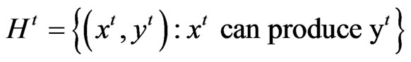
Under the assumption that each time period t = 1, 2, ..., T the production technology  models present the transformation of inputs xt, into outputs yt, as follows:
 (1)
(1)
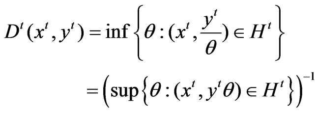
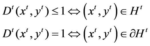
The output distance function is defined at time t as
 (2)
(2)
We have that
Here,  is the frontier of
![]() .
.
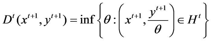
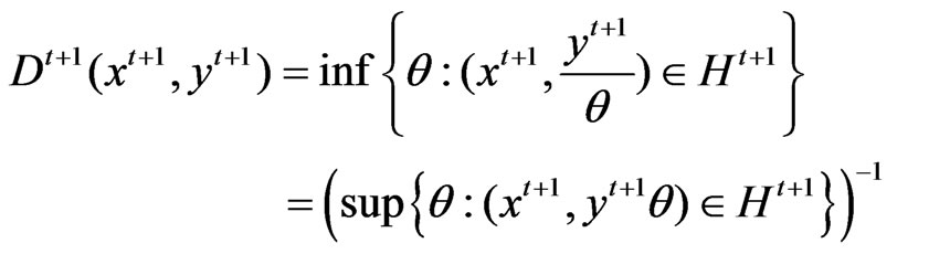
This mixed index measures the maximal proportional changes in outputs yt+1 given inputs xt+1, under the technology at time period t. Similarly, we can define the distance function with respect to two time periods as follows:
 (3)
(3)
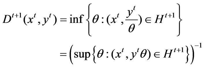
This distance function measures the maximal proportional change in outputs required to make  feasible in relation to the reference technology at time t. Similarly, a distance function that measures the maximal change in output required to make
  feasible in relation to the technology at time t+1 and distance function that measures the maximal change in output required to make
  feasible in relation to the technology at time t + 1, can be defined as follows:
 (4)
(4)
 (5)
(5)
If  then
then  and
and 
 .
.
2.1.2. The Malmquist TFP Index
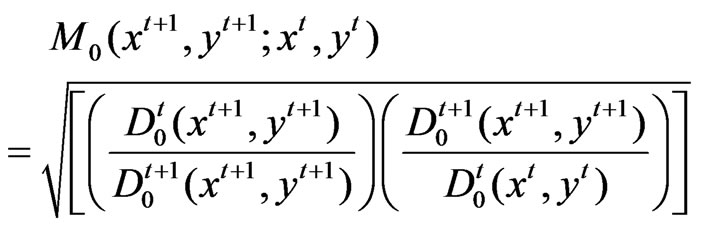
The Malmquist TFP index measures the TFP change between two data points (e.g, those of a particular province in two adjacent time periods) by calculating the ratio of the distances of each data point relative to a common technology. We specify the output-based Malmquist productivity change index as the geometric mean of two Malmquist productivity indexes, one with technology at time t and other at time t + 1 as benchmarks, as follows:
 (6)
(6)
Note that this equation is the geometric mean of two TFP indexes. The first is evaluated with respect to period t technology and the second with respect to period t + 1 technology.
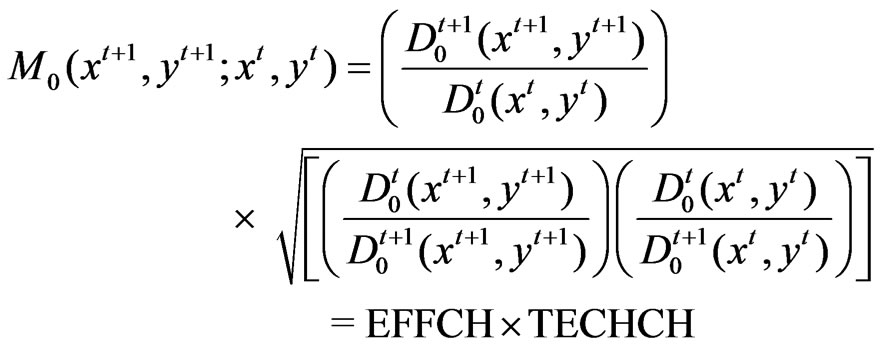
An equivalent way of writing this productivity index is:
 (8)
(8)
where EFFCH is the relative efficiency change index under constant return to scale which measures the degree of catching up to the best-practice frontier for each observation between time period t and time period t + 1 and TECHCH represents the technical change index which measures the shift in the frontier technology between two time periods evaluated at  and
and .
.
Distance functions can be estimated using various methods which differ in the type of techniques used, the type of data available, and assumptions made regarding to the economic behavior of decision makers and the structure of the production technology. In this study, we estimate the distance functions using data envelopment analysis (DEA) techniques and other modifications.
2.1.3. Data Envelopment Analysis (DEA)
Given that suitable data is available, we compute the Malmquist productivity index using non-parametric programming techniques. Assuming that there are k = 1, 2,..., K provinces that produce m = 1, ..., M outputs  using n = 1, 2, ..., N inputs at
  each time period t = 1, ..., T. The reference technology with constant return to scale at each time period t from the data can be as:
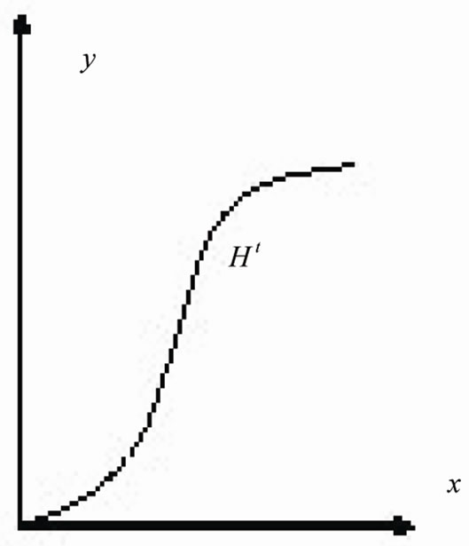
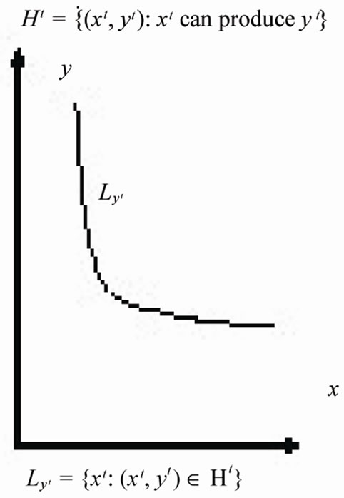
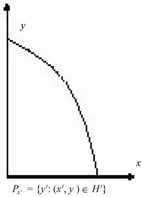
Figure 1. Production technology Ht models.
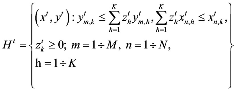
where the z are the weights on the cross-section observations.
To compute the TFP change between two periods for the kth province, four distance functions must be calculated for each province: ,
,  ,
, 
 ,
, .
.
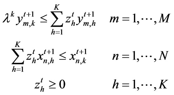
We have to solve the following four problems:
Problem 1.
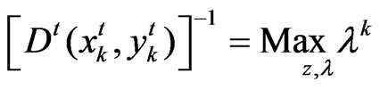
Subject to:
 (8)
(8)
Problem 2.
Subject to:
 (9)
(9)
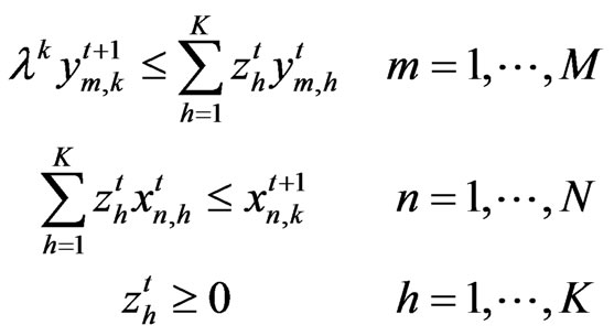
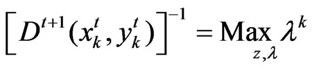
Problem 3.
Subject to:
 (10)
(10)
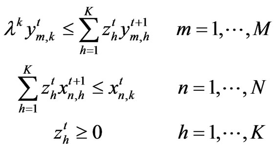
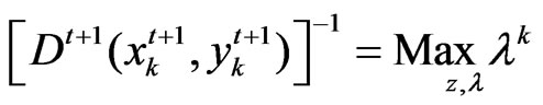
Problem 4.
Subject to:
 (11)
(11)
This approach can be further extended by decomposing the constant returns-to-scale technical efficiency change into scale efficiency and pure technical efficiency components. This involves calculating further linear program where the convexity constraint: 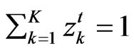 is introduced into problems (8) to (11) above. Technical change (TECHCH) is computed relative to the constant return to scale technology.
2.2. The Chanced-Constrained Programming Model and Malmquist Total Factor Productivity Index (CDEA)
2.2.1. Introduction
There have been some studies on efficiency and TFP growth using the chance-constrained programming models. Land et al. [14] examined the basic chance-constrained programming model to estimate productive efficiency in the case of stochastic inputs and outputs. Copper et al [5] developed chance-constrained programming approaches to congestion in stochastic data envelopment analysis. They incorporated the deterministic formulations used to evaluate congestion in the corresponding chance-constrained programming models. Chen [7] employed both deterministic and chance-constrained data envelopment analysis (DEA) approaches to measure the technical efficiency in Taiwan’s banks during the period of the financial crisis. He found that the 1994-1996’s deterministic DEA efficiency scores (0.924) were slightly higher than that of the 1998-2000 scores (0.909). His estimated results from deterministic DEA showed that there were certain productivity enhancements during the financial crisis period. He also showed that the chanceconstrained DEA efficiency scores were slightly higher as well as the period of technological change, but not significantly higher than efficiency scores of deterministic DEA.
Chen [8] employed both chance-constrained data envelopment analysis and stochastic frontier analysis to measure the technical efficiency of 39 banks in Taiwan. They showed that there were significant differences in efficiency scores between chance-constrained DEA and stochastic frontier production function. They also found that the ownership variable was still a significant variable to explain the technical efficiency in Taiwan, irrespective of whether a DEA, chance-constrained data envelopment analysis or stochastic frontier analysis approach was used. Gali et al. [9] developed a chance constrained programming model to assist Queensland barley growers make varietal and agronomic decision in the face of changing product demands and volatile production conditions. They showed that the analysis highlighted the suitability of chance constrained programming to this specific class of farm decision problem. Zhu et al. [10] employed chance constrained programming models for risk-based economic and policy analysis of soil conservation. They showed that chance constrained models could provide information on the trade-offs among pre-determined tolerance levels of soil loss, probability levels of satisfying the tolerance levels, and economic profits or losses resulting from soil conservation to soil conservation policy makers. They found that using chance constrained programming models, the distribution of factors being constrained had to be evaluated and if random variable followed a log-normal distribution could bias the results.
2.2.2. The Chanced-Constrained Programming Model A
The chanced-constrained programming model A based on the three assumptions:
Assumption 1: Outputs are stochastic
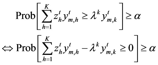
Based on the DEA models above, we suppose that the probability of the best-practice out put exceeds the observed output at least by a level a. It means that, the constraints:
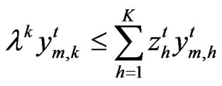 ,
, (12)
(12)
will be transformed into the constraints:
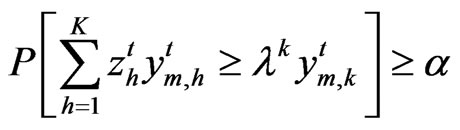 ,
, (13)
(13)
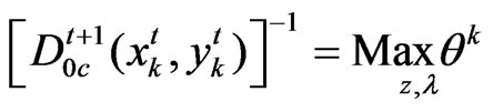
Then for the Malmquist TFP indexes with the chanceconstrained mechanisms ,
,  ,
,  ,
,  are directly derived from the above models. The chance-constrained programming models are as follows:
Problem 1*
Subject to:
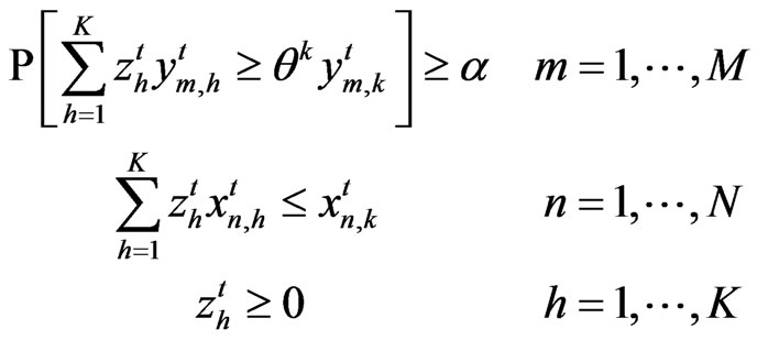 (14)
(14)
Problem 2*
Subject to:
 (15)
(15)
Problem 3*
Subject to:
 (16)
(16)
Problem 4*
Subject to:
 (17)
(17)
Here,  is a predetermined number.
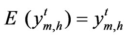
Assumption 2:  is normal distributed with mean
 , and variance
 .
.
By assuming  to be normal distributed and knowledge of the mean and variance of the distribution, this equation can be transformed into non-linear deterministic equivalents. In this case,
  is normal distributed with mean
 , and variance var
 .
.
The covariance of ,
,  is given by
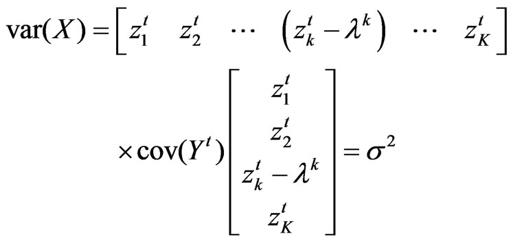
  . Consider the k constraint:
We define:
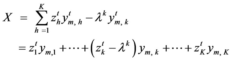
Then X is normal distributed. We assume that
Assumption 3: All outputs are stochastically independent, the performance at one province is independent of that at another province, that is  for all h = 1, 2, ..., K (it means that individual province variability of each output is the same for all outputs and at all provinces), and
 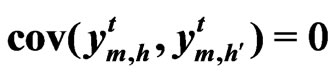 for all h≠k,
then, 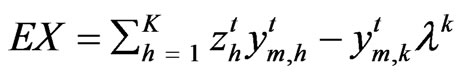 ,
,

and
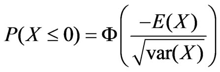
Since  is standard normal with a mean of zero and a variance of 1 (~N(0,1)).
Thus
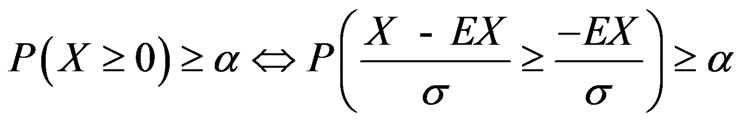
Let F be the commutative distribution function of the standard normal distribution, it means that
Let  be the standard normal value such that
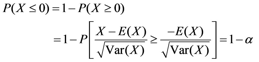
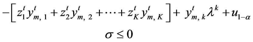
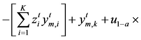
The condition
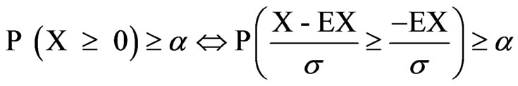
is realized if and only if
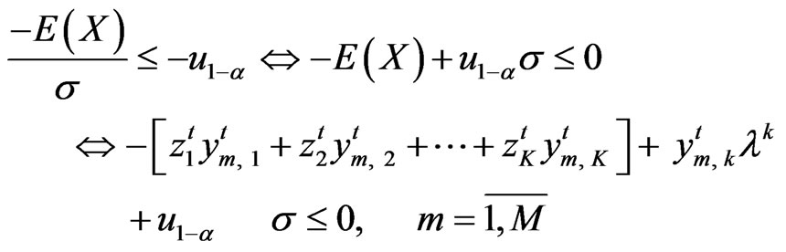 (18)
(18)
which is equivalent to the original chance constraint:
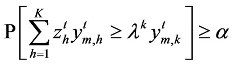
2.2.3. The Chanced-Constrained Programming Model B
The chanced-constrained programming model B based on the three assumptions:
Assumption 4: Output is stochastic (the same as model A)
Assumption 5:  is normal distributed with mean,
  and variance
 (the same as model A)
Assumption 6:  for all t for i≠s.
It means that the covariance of,  ,
,  do not depend on time. Firstly, we compute
  based on the data of outputs overtime. Secondly, we suppose
 .
.
We define 
then
By the same arguments presented above, we have
In this case, s is unknown. We use its estimate, the sample standard deviation  is:
is:
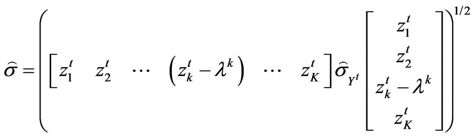
where  is the matrix of sample standard deviation of vector
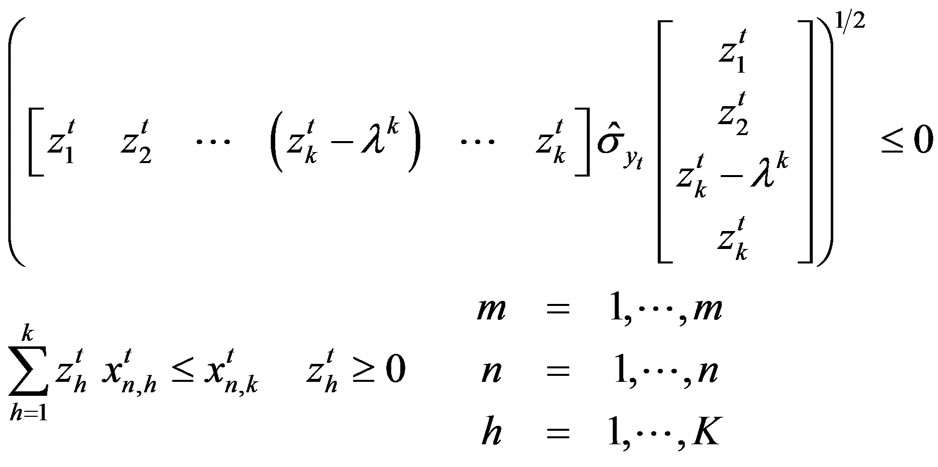
Then the constraint 
will become
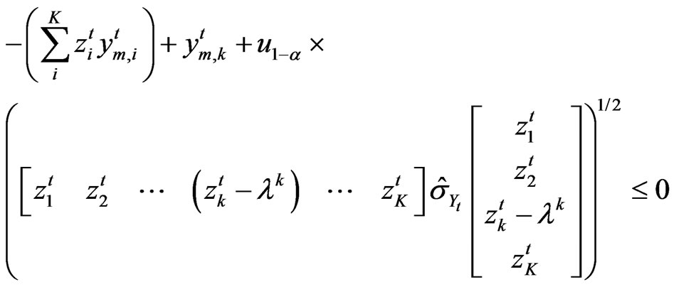 (19)
(19)
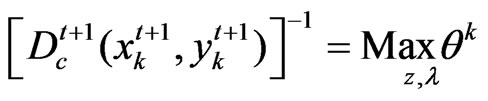
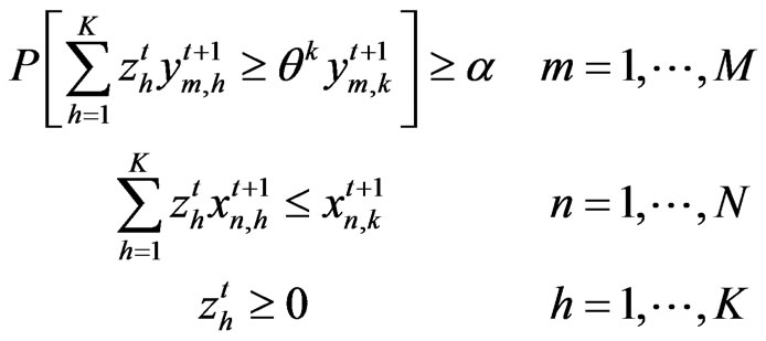
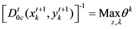
To compute the Malmquist productivity index of province k between t and t + 1, we also use the chance-constrained programming model B to calculate the following four modified distance functions ,
,  ,
,  ,
, .
.
The first of these computed for observation k given by
Subject to:
 (20)
(20)
3. Descriptive Statistics
The data used in this study are provincial-level agricultural outputs and inputs of 61 provinces in Vietnam for 1995-2007.
Data used in this study were collected mainly from Vietnamese General Statistical Office (GSO). Most of the studies on Vietnam’s agricultural efficiency or productivity used Vietnam’s gross value of agricultural output (GVA) as total value of agricultural production. Vietnam's GVA is defined as the sum of the total value of production from farming, forestry, animal husbandry, fishing, and sideline activities. The values of all inputs in agricultural production are also included in the VA. Therefore, the added value of agricultural output (VA) is used to measure the total value of Vietnam’s aggregate agricultural output in this paper. The data on provincial VA from 1995-2007 were adjusted by Vietnam’s GDP deflator (1994 = 100), which was derived from Vietnamese General Statistical Office (GSO).
The main inputs in Vietnamese agricultural production are labor, land, machinery, fertilizers, draft animals. Land refers to total cultivated areas at the end of each year. Labor (L) refers to total rural labor force in farming, forestry, animal husbandry, and sideline production but excluding the labor force in rural industry, construction, transportation, commerce, and miscellaneous occupations. Machinery (MK) refers to total power of farm machinery. It includes total mechanical power of machinery used in farming, forestry, animal husbandry, fishery, and sideline production such as plowing, harvesting, farm product processing, agricultural transport, plant protection, and stock breeding. MB refers to irrigating and draining machinery. Chemical fertilizers refer to the sum of pure or effective weight of nitrogen, phosphate, potast, and complex fertilizers.
4. Estimated Results
4.1. Classifying Models
Based on this classification of agricultural technology, we can give definitions on the models for the empirical study. The chance-constrained programming model with three assumptions 1, 2 and 3, applied for the total sample is called model A. The chance-constrained programming model with three assumptions 4, 5 and 6, applied for the total sample is called model B.
The chance-constrained programming model A or model B, applied for the sub-sample of Mekong technology (20 provinces) is called modelA20 or modelB20. The chance-constrained programming model A or model B, applied for the sub-sample of other technology (41 remaining provinces) is called modelA41 or modelB41.
Under the assumption of homogeneity technology, we have two models: the chanceconstrained programming model A and model B. In this case, we denote by effA, effchA, techchA, tfpchA and effB, effchB, techchB, tfpchB the technical efficiency, efficient change, technical change and total factor productivity change, estimated from the chance-constrained programming model A and model B, respectively.
Under the assumption of the differences in technology, we have four models: modelA20, modelA41, modelB20 and modelB41 that can be defined in the same way.
4.2. Estimated Results
We have programmed using Mathlab to solve these problems.
In this section, we present estimated results of the chance-constrained model A and model B and modification of the chance-constrained programming model A or model B. There are the chance-constrained modelA20 and modelB20 as well as the chance-constrained programming modelA41 or modelB41.
4.2.1. Estimated Results from the Chance-Constrained Programming Model A
The estimated results from the chance-constrained programming model A with homogenous technology and modelA20 and modelA41 were obtained by running 9516 non-linear programming problems for the set of input-output variables from which we get the productivity index for each provinces during the period of 1995- 2007. These results will be presented below.
4.2.1.1. Estimated Results under the Assumption of Difference in Production Technology between Mekong Technology and Other Technology
This part summaries the results obtained through chanceconstrained programming and TFP calculations from model A, model A 41 and model A 20. In this study, we decomposed the Malmquist productivity index into the technical change index (techch) and efficiency change (effch) index. To obtain the Malmquist productivity indexes for each province and each pair of years, we used stochastic constrained programming modelA to compute.
Before presenting the disaggregated results for each region and each province, we present the average annual changes of Malmquist productivity indexes and their components for Mekong technology provinces and other technology provinces over the 1995-2007 period in Table 2.
Recalling that tfpch indicates the degree of productivity change, then if tfpch > 1 the productivity gains occur, whilst if tfpch < 1 productivity losses occur. The estimated results showed that the average productivity growths in agricultural production were at –0.1 and –0.7 percent for provinces with other technology and Mekong technology, respectively. Given that tfpch is a multiplicative composite of effch and techch, the major cause of productivity improvements can be ascertained by comparing the values of the efficiency change and technological change indexes. Put differently, the productivity improvement described can be the result of efficiency gains, technical progress, or both (I do not understand this sentence).
In the case of other-technology provinces, the overall decrease in productivity over the period is composed of an average efficiency (movement away from the frontier) of 0.5 percent, and average technological progress (downward shift of the frontier) of –0.1 percent.
In the case of Mekong-technology provinces, the decline in productivity over the period is composed of an average efficiency increase by 0.2 percent, and average technological progress (downward shift of the frontier) of –0.7 percent.
Growths in technical change and in technical efficiency suggest that increased total factor productivity in other-technology provinces arose from both the innovation in technology and improvement in technical efficiency.
Decline in technical efficiency (0.5 percent) and increase in technical progress (0.5 percent) suggest that decreased total factor productivity in other technology provinces from the declining in technical efficiency.
Among the total 41 provinces in the other technology provinces, eighteen provinces: Hanoi, Vinh Phuc, Hai Duong, Cao Bang, Lao Cai, Thai Nguyen, Quang Ninh, Nghe An, Quang Tri, Thua-Thien-Hue, Da Nang, Quang Nam, Quang Ngai, Binh Dinh, Phu Yen, Gia Lai, Dak Lak, Lam Dong had positive average growth rates in total productivity during 1995-2007 period.
Bac Ninh, Ha Tay, Ha Nam, Nam Dinh, Tuyen Quang, Lai Chau were provinces with negative growths in technical change, as well as in other indexes, while Hanoi, Lao Cai, Thai Nguyen, Quang Ninh, Quang Ngai, Binh Dinh were the provinces which had improvements in all indexes.
Among the Mekong-technology provinces, Binh Duong, Ben Tre, Soc Trang had the greatest decline in total factor productivity since their poorest performance in technical change and low technical efficiency change.
We compare the mean tfpch for Mekong technology group and other technology group. We found that efficiency change of Mekong technology group was better than the other technology group.
4.2.1.2. Estimated Results under the Assumption of Uniform Technology between Two Regions Malmquist Indexes
Before presenting the disaggregated results for each province, we turn to a summary description of the average performance of all provinces. Looking first at the
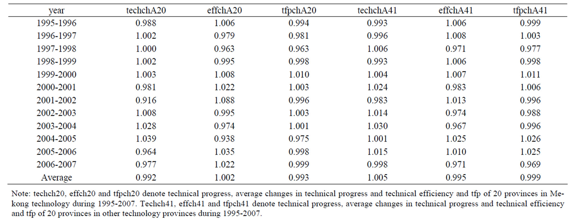
Table 1. Malmquist TFP results: annual sample mean (from model A).
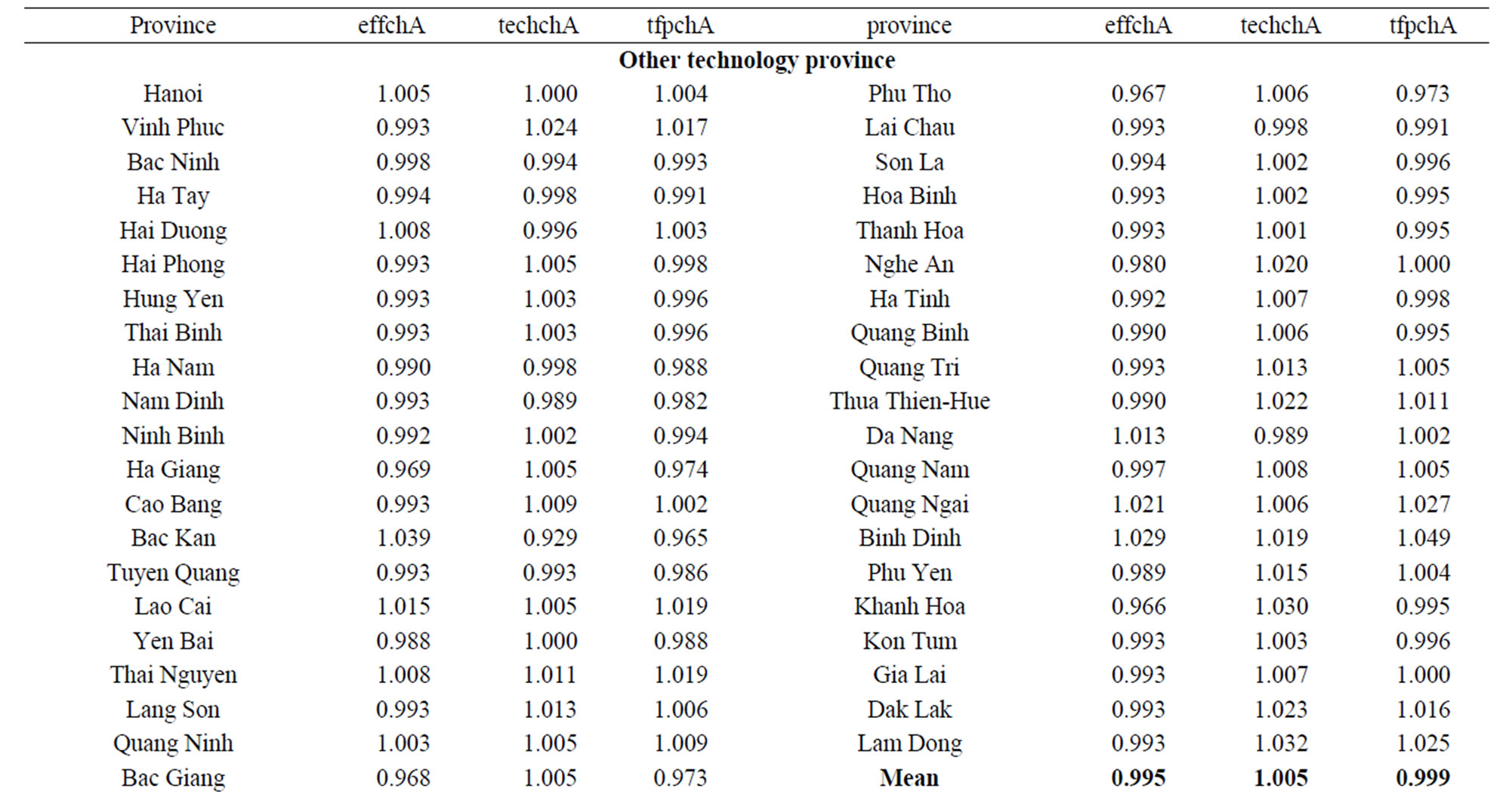
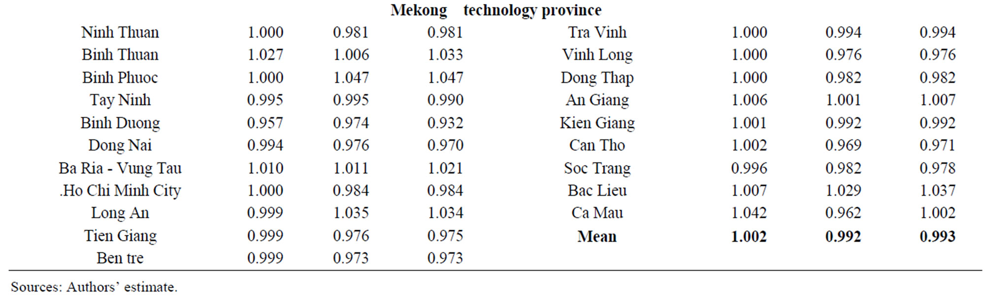
Table 2. Malmquist index summary of province means (Output-Oriented Measured) (From chance-constrained programming model A).
tfpch columns of Table 3, we see that productivity increased slightly in years 1997, 2001, 2002, 2003 and 2004. The values of Malmquist indexes in 1997, 2001 and 2003 were greater than 1 because of improvements in the technical efficiency. While the value of Malmquist index in 2004 was greater than 1 because of the improvements in the technical progress Turning to the variation of TFP within the sample for individual provinces is even more striking as can be seen in the Table 5.
Dak Lak, Binh Phuoc experienced the highest growth in both total productivity and technical change, followed by Lam Dong, Binh Dinh, Ha Nam and Ninh Binh had the largest improvement in technical progress, but it also showed a large decline in technical efficiency. (This sentence should be rewritten).
Ca Mau, An Giang, Quang Ninh and Son La had the largest gain in technical efficiency, while their technical progresses suffered the great decline. Thai Binh is the largest agricultural province in other technology category, experienced the large fall in technical progress.
4.2.2. Estimated Results from the Chance-Constrained Programming Model B
This part summaries the results obtained through the chance-constrained programming and TFP calculations from model B, modelB41 and modelB20. The disaggregated results for each region and province in Mekong technology provinces and other technology provinces over the 1995-2007 period are given in Table 6.
The estimated results from the model B show that the average productivity growths in agricultural production
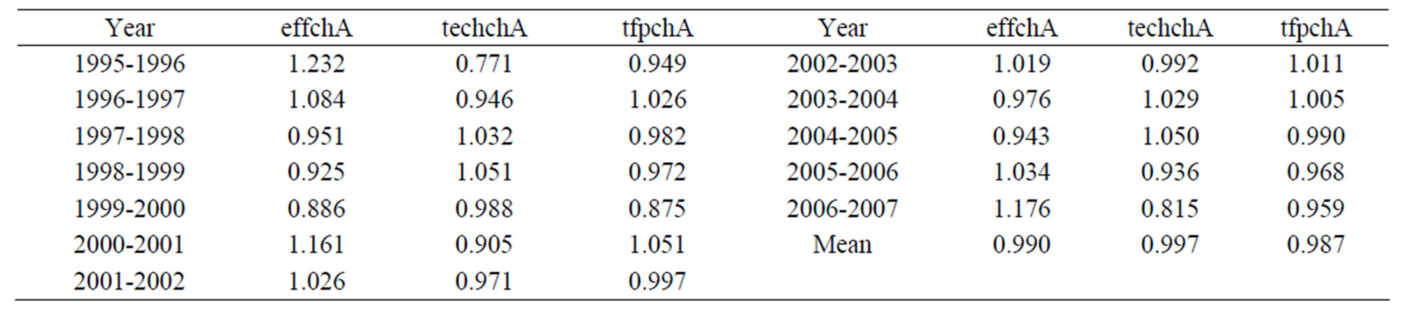
Table 3. Malmquist TFP results: annual sample averages.
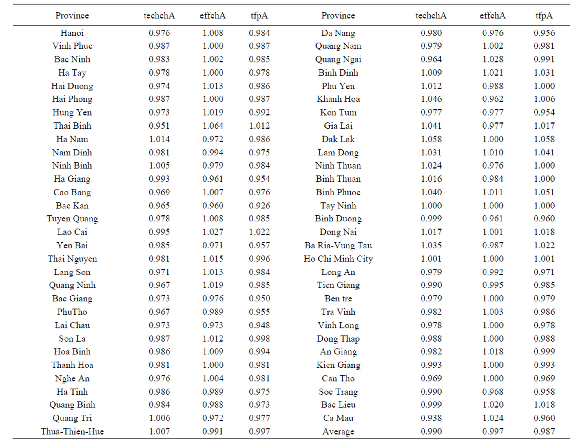
Table 4. Average annual changes of Malmquist indexes under homogenous technology by provinces, 1995-2007 (Output-oriented) from chance-constrained programming model A.
are at –1.3 and 0 percent for provinces with other technology and Mekong technology, respectively.
In the case of other-technology provinces, the overall decrease in productivity over the period is due to the decline in technical efficiency (1.4 percent).
In the case of Mekong-technology provinces, unchanged in productivity over the period is composed of an average efficiency increase in technology progress by 0.1 percent, decrease in technical efficiency by 0.1 percent. (This sentence should be changed)
Among the total 41 provinces in the other technology provinces, eight provinces: Ha Tay, Cao Bang, Tuyen Quang, Lang Son, Quang Binh, Da Nang, Khank Hoa, Gia Lai and Lam Dong had negative average growth rates in technological progress during 1995-2007 period.
Hanoi, Bac Ninh, Hai Duong, Ninh Binh, Lao Cai, Yen Bai, Thai Nguyen Son La, Hoa Binh, Ha Tinh, Quang Tri Quang Ngai, Binh Dinh, Phu Yen, Kon Tum
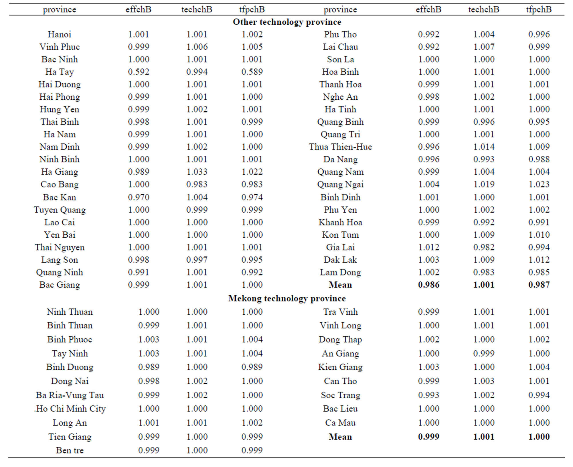
Table 5. Malmquist index summary of province means (Output-Oriented Measured) (From chance-constrained programming model B).
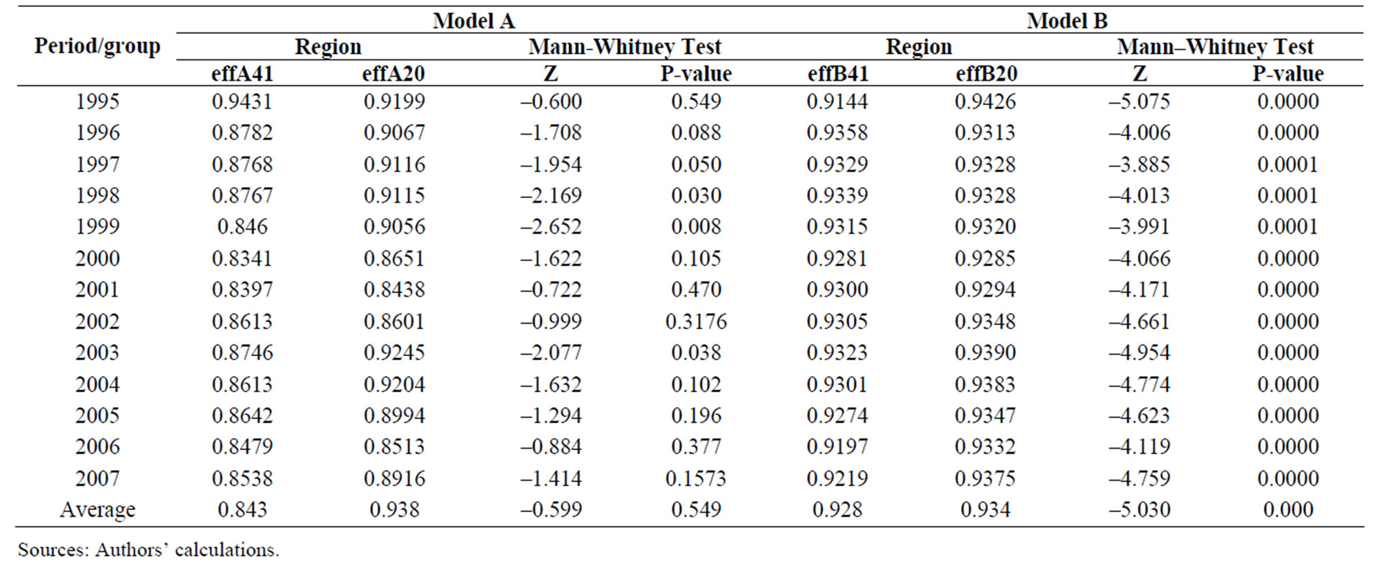
Table 6. Mean efficiency and mann-whitney test.
and Dak Lak had improvements in all three indexes.
Among the Mekong-technology provinces, Ninh Thuan, Binh Phuoc, Tay Ninh, Ho Chi Minh City, Long An, Vinh Long, Dong Thap, Ang Giang, Kien Giang, Bac Lieu and Ca Mau had improvement in all three indexes.
In other technology, Bac Kan, Lang Son, Quang Ninh, Phu Tho, and Da Nang and Binh duong, Soc Trang in Mekong technology had the greatest decline in total factor productivity since their poorest performances in technical efficiency change.
4.3. Comparing Technical Efficiency between two Technologies under the Assumption of Different Technologies
4.3.1. Comparing Technical Efficiency between Mekong Technology Provinces and Other Technology Provinces from Chanced-Constrained Programming Model A and Model B
In this part, we conduct a Mann-Whitney test to verify whether the two samples above (Mekong technology province sample and other technology sample) were drawn from the same productivity change populations. The Mann-Whitney test is one of the non-parameter statistical methods used to test the same mean between two groups.
The results of Mann-Whitney test for each period, estimated from model A and model B are presented in the Table 7 below.
The fifth column of Table 5 shows that the Mekong technology category and the other technology category are not significantly different in the years 2000, 2001, 2002, 2004, 2005, 2006, 2007 and average efficiency, except for 1995, 1996, 1997, 1998, 1999, 2003, from the chance-constrained programming modelA20 and modelA40. (This sentence should be changed).
From the chance-constrained programming model B, the p-value of Mann-Whitney test presented in the last column indicates that the differences between the Mekong technology category and other technology category are more significant. They are significantly different at 1% level 0.
4.3.2. Detecting Stable Efficiency Rakings under the Assumption of Homogenous Technology from the Chance-Constrained Model A and Model B
4.3.2.1. Average Technical Efficiency from Two Models
The results of estimating average technical efficiency from the chance-constrained model A and model B are presented in Table 8. Estimated results show that there is a large variation in the estimated derived.
Estimated results from the chance-constrained programming model A are more variation than those from model B. The minimum estimate is 0.4882 during for the period of studying, while the overall provinces average recorded during the period is at 0.8479.
For the chance-constrained model B, the estimated results is a small variation (This should be changed). The minimum estimate is 0.7901, while the maximum estimate is only 0.9295
Table 8 illustrates the frequent distributions of average technical efficiency over period of 1995 - 2007 from two models. The mean technical efficiencies of four out of thirteen years from the model A and model B fall within the ranges of 82% - 84% and 90% - 91%, respectively.
4.3.2.2. Detecting the Stability of Efficiency Ranking between Provinces from Two Models
From the estimated results, we observed that while some provinces exhibit an upward trend in their efficiency

Table 7. Average technical efficiency scores during 1995- 2007 estimated from two models.
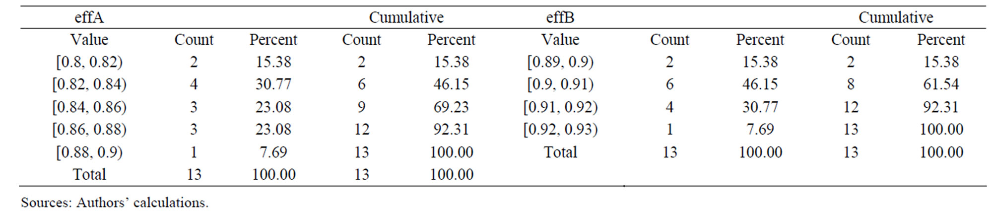
Table 8. Frequency distribution of average technical efficiency from two models.
ratings during the period of 1995-2007, most of the provinces do not seem to consistently conform to such a trend.
We apply Kruskal-Wallis Non-parametric Analysis of Variance (ANOVA) test to find the relative efficiency rank position between provinces.
For this test, there are N “populations” (or 61 provinces in this study) and 13 years (K), simultaneously under investigation and the null hypothesis is that all N “populations” have the same distribution of ratings. This test statistic is distributed according to a x2 distribution with (N-1) degree of freedom.
The values of the Kruskal-Wallis test statistic that correspond to the overall ranks from the chance-constrained model A and the chance-constrained model B are H = 592.85 and 623.04, respectively which, when compared to  = 91.9517 does allow the rejection of the null hypothesis of identical distribution of efficiency ranking for all 61 provinces at a level of significance 0.005. Our estimated mean values of technical efficiency from both approaches for some provinces are higher than those of them in the study period.
From Table 9 and by using their overall sum-of-ranks from the chanced-constrained programming model A, the 61 provinces can be ordered from the highest to lowest ranks as follow: Vinh Long, Ben Tre, Kien Giang, Tay Ninh, Thai Binh, Hai Phong and Tien Giang. Similarly, by using their overall sum-of-ranks from the chancedconstrained programming model B, the 61 provinces can be ordered as: Vinh Long, Kien Giang, Tien Giang, Thai Binh, Dong Nai, Ben Tre, and An Giang. This means that Vinh Long exhibited the overall largest average rank from both models.
4.4. Comparing Chanced-Constrained Programming Model A and Model B Results
The two models used here to decompose TFP growth into technical efficiency change and technical progress from the sample production of the provinces are based on the differences in the third assumption.
4.4.1. Testing for the Efficiency Differences between the Stochastic-Constrained Programming Model A and Model B
In this part we consider two types of models: a) the stochasticconstrained programming model A and model B for the whole sample; b) the stochasticconstrained programming model A and model B for the Mekong technology with the sample size to be 20; the stochasticconstrained programming model A and model B for the other technology with the sample size to be 41. The agreements or disagreements in the efficiency scores estimated from these two types of models can be examined by using banker’s asymptotic DEA efficiency tests and Welch’s mean test. These results are presented in
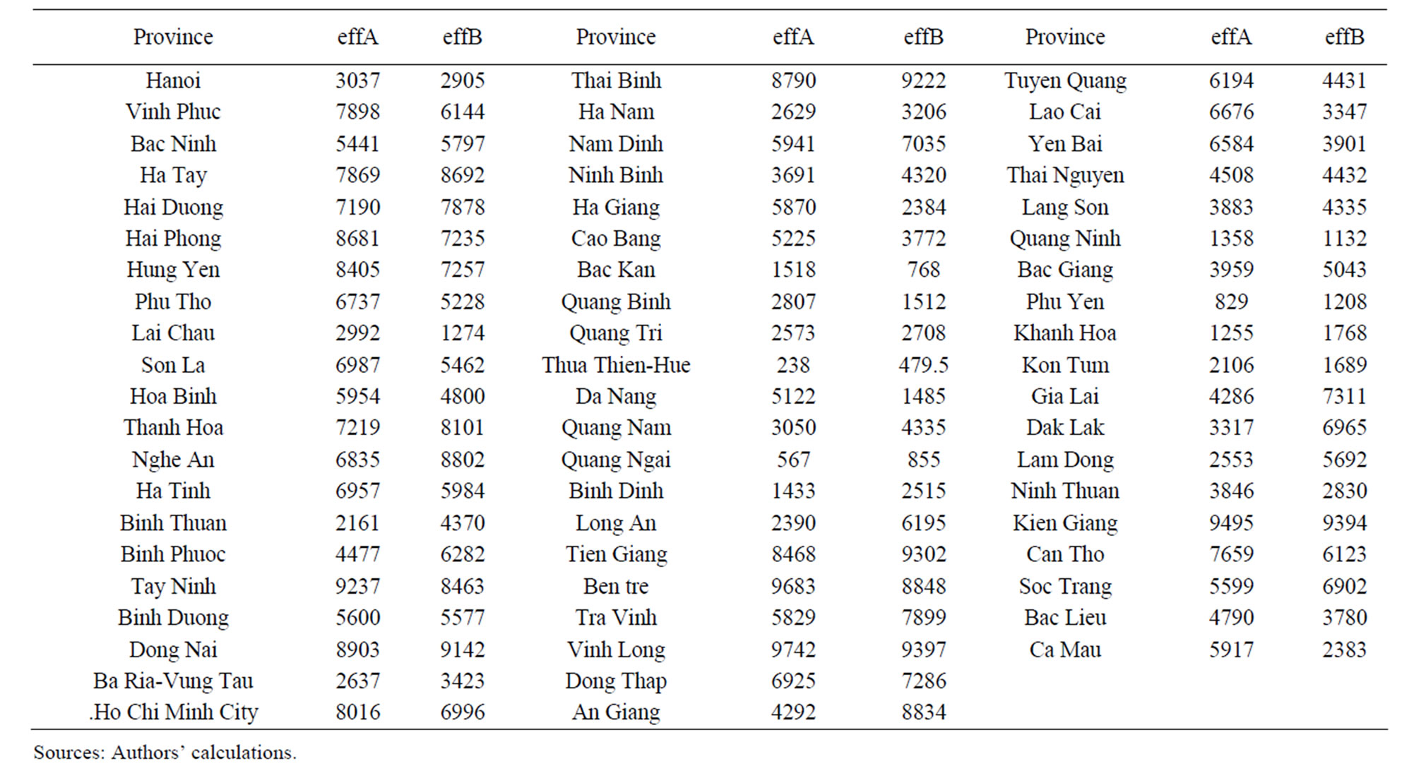
Table 9. Some of rank matrix for province productivity over time.
Table 10.
The computed results from the Table 10 show that the chance-constrained programming model A measurements have a different efficiency score from the chanceconstrained programming model B, except the chanceconstrained modelA20 and the chance-constrained modelB20. As it can be seen from the Table 10, only one case of Me Kong technology, Banker’s DEA test with the exponential type the F-statistics (1.627) is less than the critical value (1.69), so the chance-constrained modelA20 measurement does not have a different efficiency score from the chance-constrained modelA20 measurement.
4.4.2. Comparing the Malmquist Indexes Estimated from Two Models for Period 1995-2007
The agreements or disagreements in the total factor productivity indexes and their components estimated from two models: the stochastic-constrained programming model A and model B will be examined in this part.
For comparison, we also calculate the Malmquist indexes based on the assumption of homogenous technology for all 61 provinces (in Table 12) and Figure 2.
Figure 2 shows the evaluation of average Malmquist indexes during the period of studying from different models. Efficiency, technological and total factor productivity change estimated from two models seem to be different from each other. However, tfpch index from the chance-constrained model B is more stable than those from the chance-constrained model A. We can see that the three lines: techchB, effchB and tfpchB from model B almost coincide, which indicates that the change in TFP from two model B has been impacted by changes in both technical and efficiency during 1995-2007.
However, this is not the case for the components in the decompositions of the Malmquist indexes from model A. The measure techchA show much more volatility than what of the techchB.
In the Table 11 we compute the Malmquist indexes and the corresponding technical change and efficiency change components for periods 1995-2007 from two models.
As indicated in Table 12, there was a mean annual decrease in total factor productivity of 0.13 percent for model A and 0.031 percent for model B over the period 1995-2007. Given that the Malmquist index of productivity change (tfpch) is a multiplicative composite of efficiency change (effch) and technological change (techch), the major cause of productivity decrease can be scertained by comparing the values of the efficiency
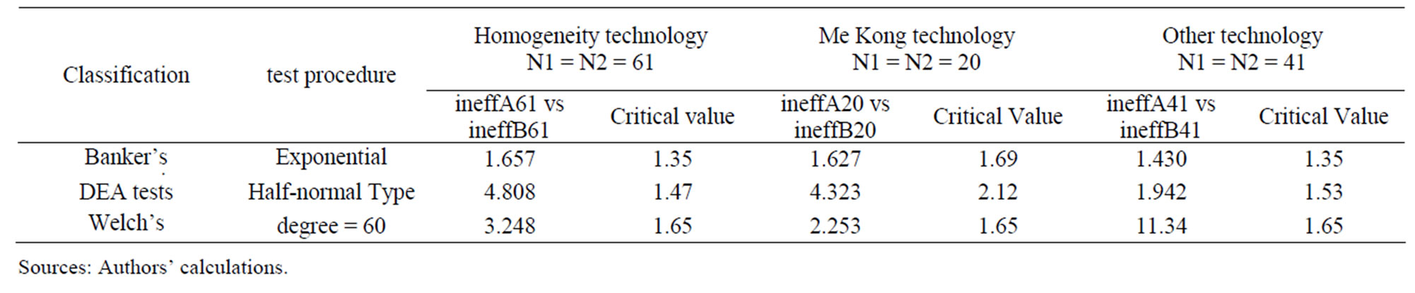
Table 10. Summary of efficiency difference test results from the chance-constrained model A and the chance-constrained model B.
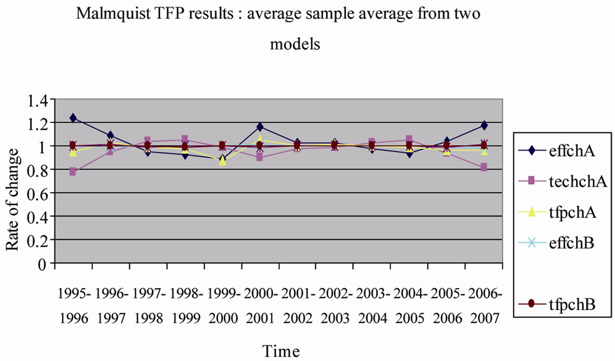
Figure 2. Malmquist TFP results from two models.
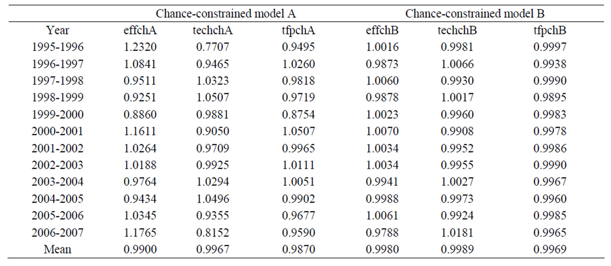
Table 11. Malmquist index summary of annual means from two models, for period 1995-2007.
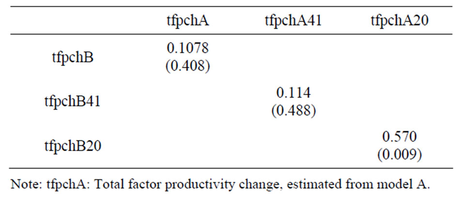
Table 12. Summary of correlation between the alternative Malmquist indexes.
change and technological change indexes.
In the case of model B, the overall decrease (0.031 percent) in productivity over the period 1995-2007 is composed of an average efficiency decrease 0.02 percent, and average decrease in technical change of 0.11 percent.
In the case of model A, the overall improvements in productivity over the periods 1996-1997, 2000-2001, 2002-2003 are composed of an average efficiencies increase of 8.8, 16.11, 1.88 percents and average decrease in technical changes of 0.535, 0.95, 0.7 percents, respectively. But the overall improvement in productivity over the periods 2003-2004 is composed of an average efficiency decease of 0.236 percent and average technological progress of 2.94 percent.
Table 12 summaries the correlation between the Malmquist indexes from models A, modelA41, modelA20 and model B, modelB41 and modelB20.
From the table, we observe that although the correlation between Malmquist indexes is positive, it is not very high, except tfpchA20 and tfpchB20. It shows that they are much less correlation. Thus, there is little discrepancy between the two Malmquist indexes estimated from chance-constrained model A and model B since the chance-constrained frontier of models A and B are different.
5. Conclusions
In this paper an attempt has been made to assess the agricultural total factor productivity by province via six models: the chance-constrained programming modelA, modelA20, modelA41 and model B, modelB20, modelB41 and compares the efficiency, total factor productivity estimates obtained from the models.
According to the regional characteristics of agricultural production in Vietnam was classified into Mekong technology and other regional technology categories. The Malmquist index was used to measure productivity growth in this study.
The primary objective in this study is to decompose the total factor productivity change of Vietnamese agriculture by province into technical change and technology progress by using the chance-constrained programming models with two kinds of assumptions. This decomposition allows us to identify the contributions of technical change and improvement in technical efficiency to productivity growth in Vietnamese production.
The results from estimated technical efficiency suggest that, over the data period, some provinces operated at or near frontier in at least some of years studies. Moreover, the average technical efficiency in the most year is around 0.8 to 0.9 from two models. Our results indicate that there are significant statistical differences between technical efficiency estimates across years in the panel. There are substantial differences in overall performance between provinces. The potential production differences between the highly efficient provinces and the least efficient are generally consistent with the potential for an increasing output on the less efficient provinces without changing the level of their input use.
The results from the Kruskal-Wallis test statistic suggest that we reject the null hypothesis of identical distribution of efficiency ranking for all 61 provinces at a level of significance 0.005 and some of the provinces exhibited consistently better economic performance than the others.
Other finding of this study shows that during the thirteen sample years, TFP growth estimated from two models (the chance-constrained programming model A and model B) was dominant in the Ho Chi Minh City. This was mainly due to technical change rather than efficiency change from model A and due to both technical change and efficiency change from model B.
The Malmquist results also show that production frontier has contracted by around 1.3 percent and 0.31 percent from the chance-constrained model A and model B, respectively, a year on average over the sample period. This results can be explained by substantial changes that occurred in 1995-1996, 2000-2001 from both models.
The decline in productive potential could be explained by a general reduction in the quality of managerial decision-making among best practice provinces, infrastructure or irrigation system or climate change....
General conclusion from this study is that in the agricultural sector technical change or exploiting advanced technology is critical for each province. Knowledge and innovation can play an important role in increasing technical efficiency in an organization’s production processes.
6. References
[1] W. Mao and W.W. Koo, “Productivity Growth, Technological Progress, and Efficiency Change in Chinese Agriculture after Rural Economic Reforms: A DEA Approach,” China Economic Review, Vol. 8. No. 2, 1997, pp. 157-174. doi:10.1016/S1043-951X(97)90004-3
[2] M. Nishimizu and J. M. Page, “Total Factor Productivity Growth, Technological Progress and Technical Efficiency Change: Dimensions of Productivity Change in Yugoslavia, 1965-1978,” The Economic Journal, Vol. 92, No. 368. 1982, pp. 920-936. doi:10.2307/2232675
[3] N. K. Minh and G. T. Long, “Factor Productivity and Efficiency of the Vietnamese Economy in Transition,” Asia-Pacific Development Journal, Vol. 15, No.1, 2008, pp. 93-117.
[4] A. Charnes and W. W. Cooper, “Chance-Constrained Programming,” Management Science, Vol. 6, No.1, 1959, pp. 73-79. doi:10.1287/mnsc.6.1.73
[5] W. W. Copper, H. Deng, Z. Huang and S. X. Li., “Chance Constrained Programming Approaches to Congestion in Stochastis Data Envelopment Analysis,” European Journal of Operation Research, Vol. 155, No. 2, 2004, pp. 487-501. doi:10.1016/S0377-2217(02)00901-3
[6] W. W. Copper, Z. Huang, V. Lelas, S. X. Li and O. Olesen, “Chance Constrained Programming Formulations for Stochastic Characterizations of Efficiency and Dominance in DEA,” Journal of Productivity Analysis, Vol. 9, No.1, 1998, pp. 53-79. doi:10.1023/A:1018320430249
[7] T. Chen, “A Measurement of Taiwan’s Bank Efficiency and Productivity Change during the Asian Financial Crisis,” International Journal of Services Technology and Management, Vol. 6, No. 6, 2005, pp. 525-543. doi:10.1504/IJSTM.2005.007510
[8] T. Chen, “A Comparison of Chance-Constrained DEA and Stochastic Frontier Analysis: Bank Efficiency in Taiwan,” The Journal of the Operational Research Society, Vol. 53, No. 5, 2002, pp. 492-500. doi:10.1057/palgrave.jors.2601318
[9] V. J. Gali and C. G. Brown, “Assisting DecisionMaking in Queensland Barley Production through Chance Constrained Programming,” The Australian Journal of Agricultural and Resource Economics, Vol. 44, No. 2, 2000, pp. 269-287. doi:10.1111/1467-8489.00111
[10] M. Zhu, D. B. Taylor, S. C. Sarin and R. A. Kramer, “Chance Constrained Programming Models for Risk Based Economic and Policy Analysis of Soil Conservation,” Agricultural and Resource Economics Review, Vol. 23, No. 1, 1994, pp. 58-65.
[11] J. Zheng and A. Hu, “An Empirical Analysis of Productivity in China (1997-2001),” Journal of Chinese Economic and Business Studies, Vol. 4, No. 3, 2006, pp. 221- 239. doi:10.1080/14765280600991917
[12] D. W. Caves, L. R. Christensen and W. E. Diewert, “Multilateral Comparisons of Output, Input and Productivity using Superlative Index Numbers,” The Economic Journal , Vol. 92, No. 365, 1982, pp. 73-86. doi:10.2307/2232257
[13] R Färe, S. Grosskopf, M. Norris and Z. Zhang, “Productivity Growth, Technical Progress and Efficiency Change in Industrialized Countries,” The American Economic Review, Vol. 84, No. 1, 1994, pp. 66-83.
[14] K. C. Land, C. A. Knox Lovell and S. Thore “ChanceConstrained Data Envelopment Analysis,” Managerial and Decision Economics, Vol. 14, No. 6, 1993, pp. 541- 554. doi:10.1002/mde.4090140607
[15] M. J. Farrell, “The Measurement of Productive Efficiency,” Journal of the Royal Statistical Society, Vol. 120, No. 3, 1957, pp. 253-290. doi:10.2307/2343100
[16] J. Felipe, “Total Factor Productivity Growth in East Asia: A Critical Survey,” The Journal of Development Studies, Vol. 35, No.4, pp. 1-41. doi:10.1080/00220389908422579
[17] K. P. Kalirajan, M. B. Obwona and S. Zhao, “A Decomposition of Total Factor Productivity Growth: The Case of Chinese Agricultural Growth before and after Reforms,” American Journal of Agricultural Economics, Vol. 78, No.2, 1996, pp. 331-338. doi:10.2307/1243706
[18] S. Kim and G. Han, “A Decomposition of Total Factor Productivity Growth in Korean Manufacturing Industries: A Stochastic Frontier Approach,” Journal of Productivity Analysis, Vol. 16, No 3, 2001, pp. 269-281. doi:10.1023/A:1012566812232
[19] J. Kim and L. J. Lau, “The Source of Economic Growth of the East Asian Newly Industrialized Countries,” Journal of the Japanese and International Economies, Vol. 8, No.3, September 1994, pp. 235-271. doi:10.1006/jjie.1994.1013
[20] J. Kim and L. J. Lau, “The Source of Asian Pacific Economic Growth,” The Canadian Journal of Economics, Vol. 29, Apr 1996, pp. 5116-5154.
[21] B. L. Miller and H. M. Wagner, “Chance-Constrained Programming with Joint Constraints,” Operations Research, Vol. 13, No. 6, 1965, pp. 930-945. doi:10.1287/opre.13.6.930
[22] O. B. Olesen and N. C. Petersen, “Chance Constrained Efficiency Evaluation,” Management Science, Vol. 41, No. 3, 1995, pp. 442-457. doi:10.1287/mnsc.41.3.442
Appendix A: DEA Results
This part summaries the results obtained through DEA results and TFP calculations.
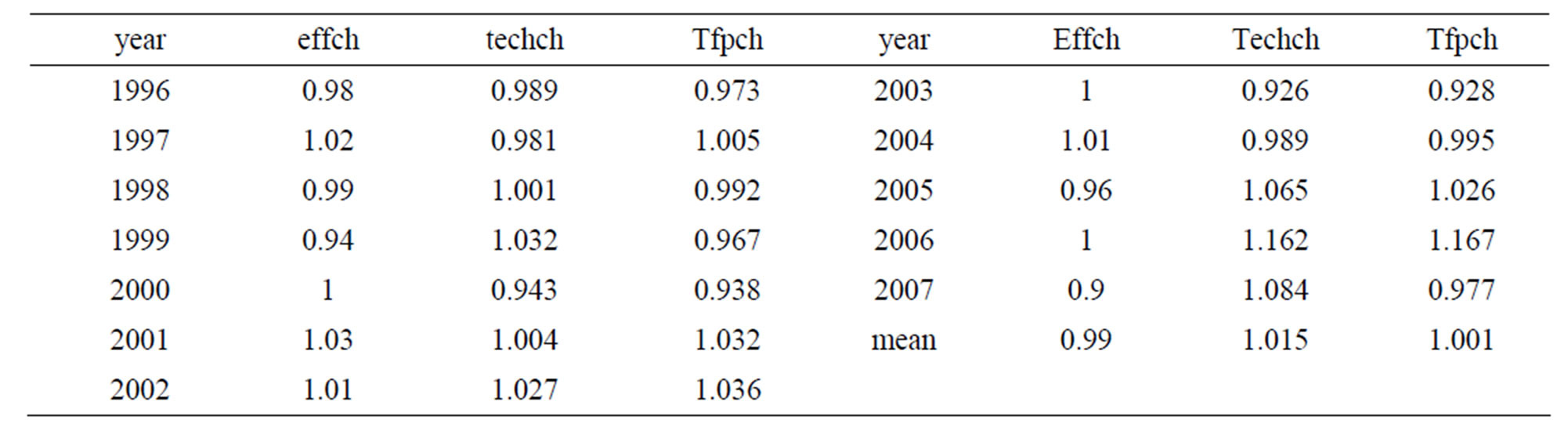
Table A1. Malmquist TFP results: annual sample averages.
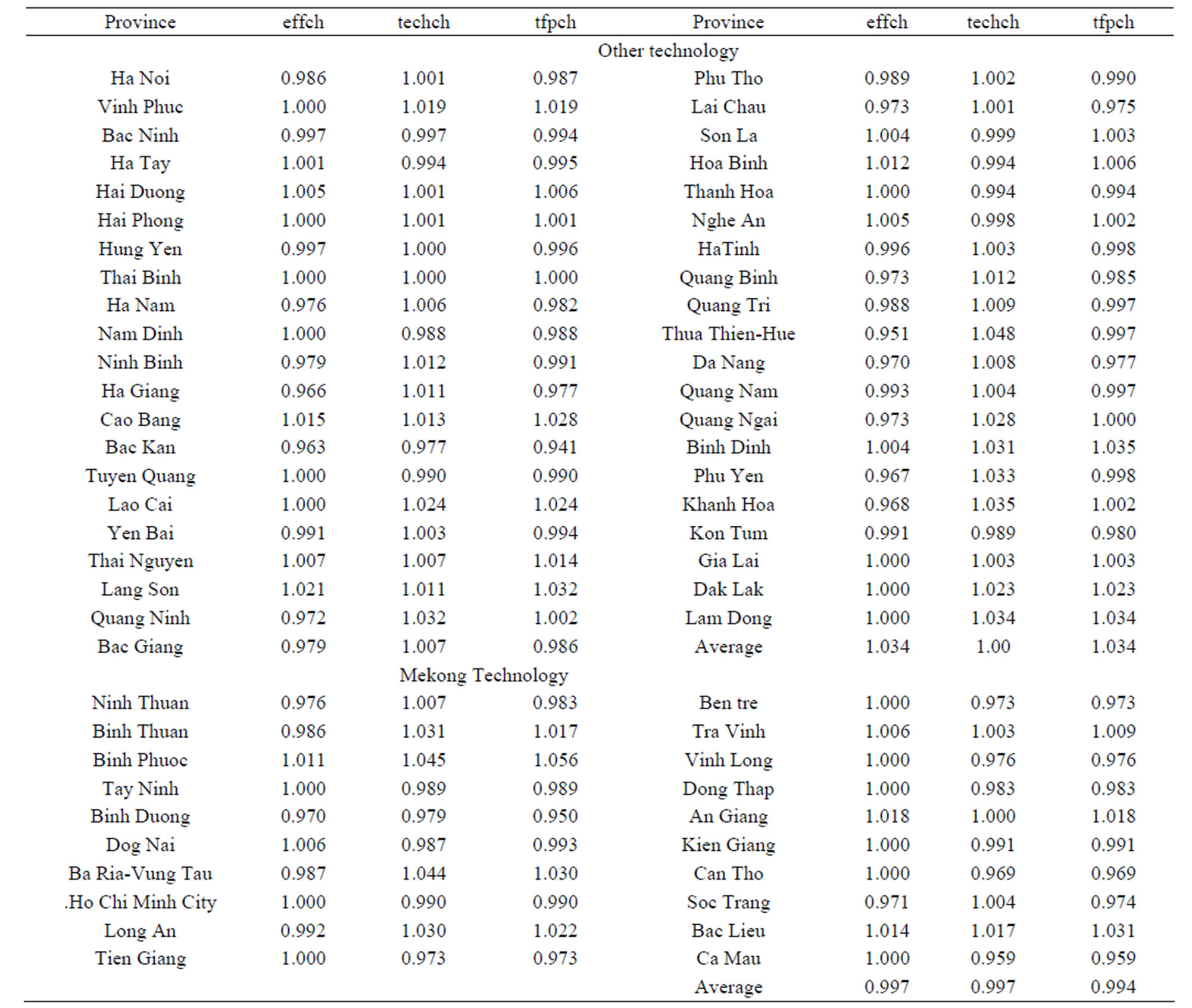
Table A2. Malmquist index summary of province means from DEA results (Output-Oriented Measured).
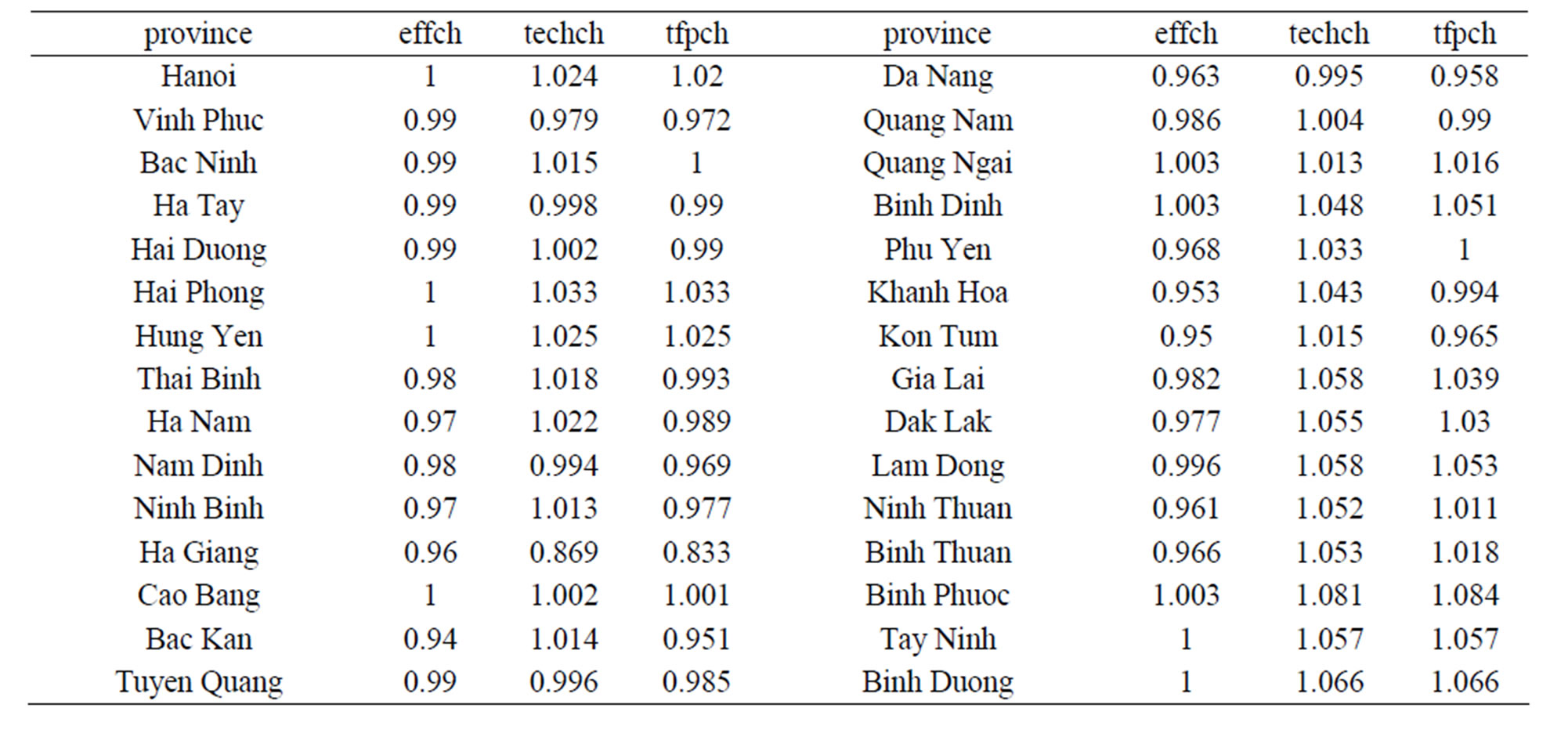
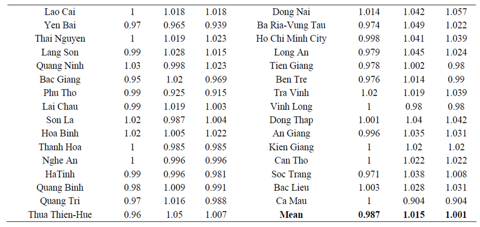
Table A3. Average annual changes of Malmquist indexes under homogenous technology by provinces, 1995-2007 (Outputoriented) from DEA results.
Appendix B: Estimated Results from Chance-Constrained Programming Model B
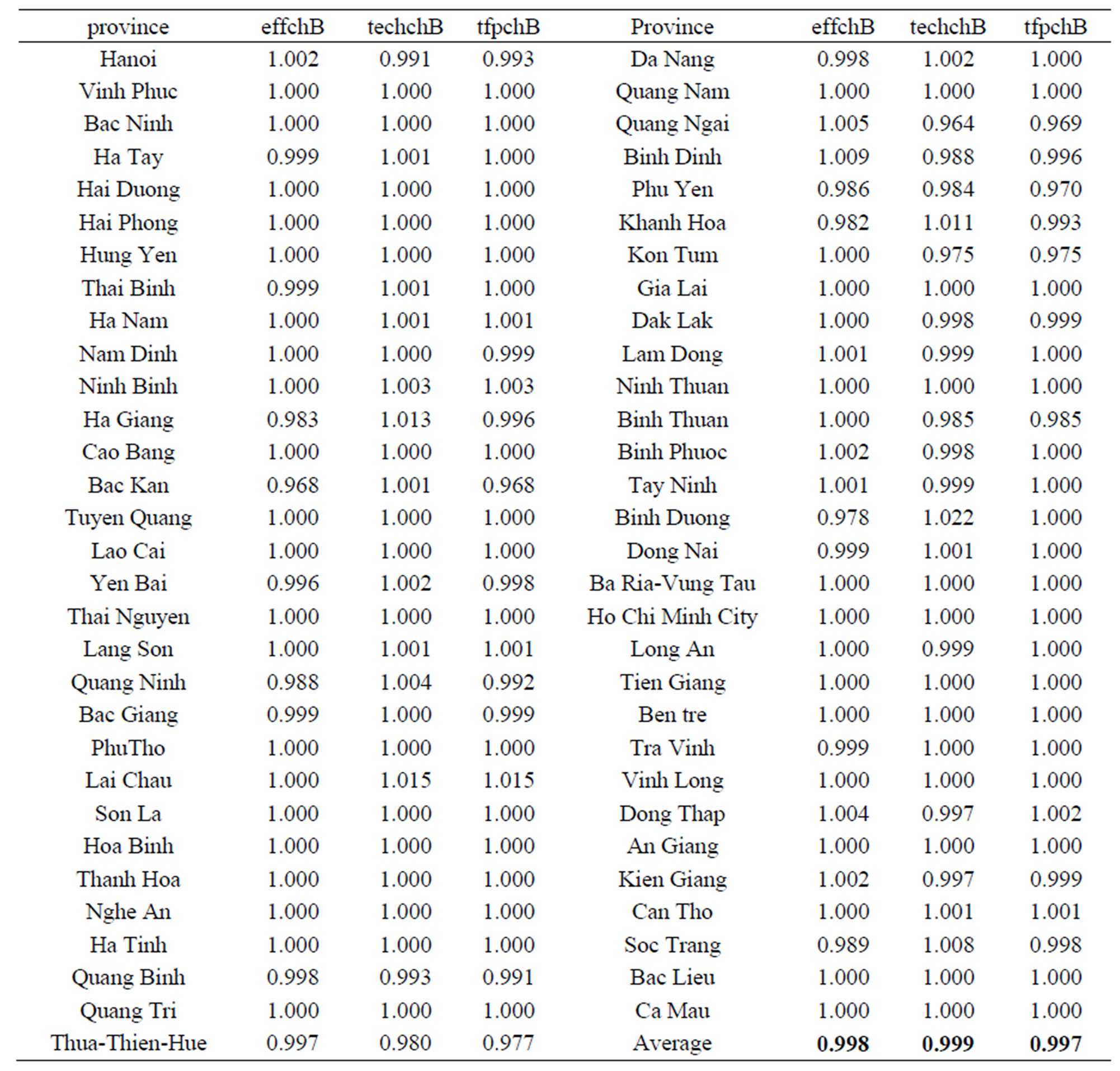
Table B1. Average annual changes of Malmquist indexes under homogenous technology by provinces, 1995-2007 (Output - oriented) from chance-constrained programming model B.