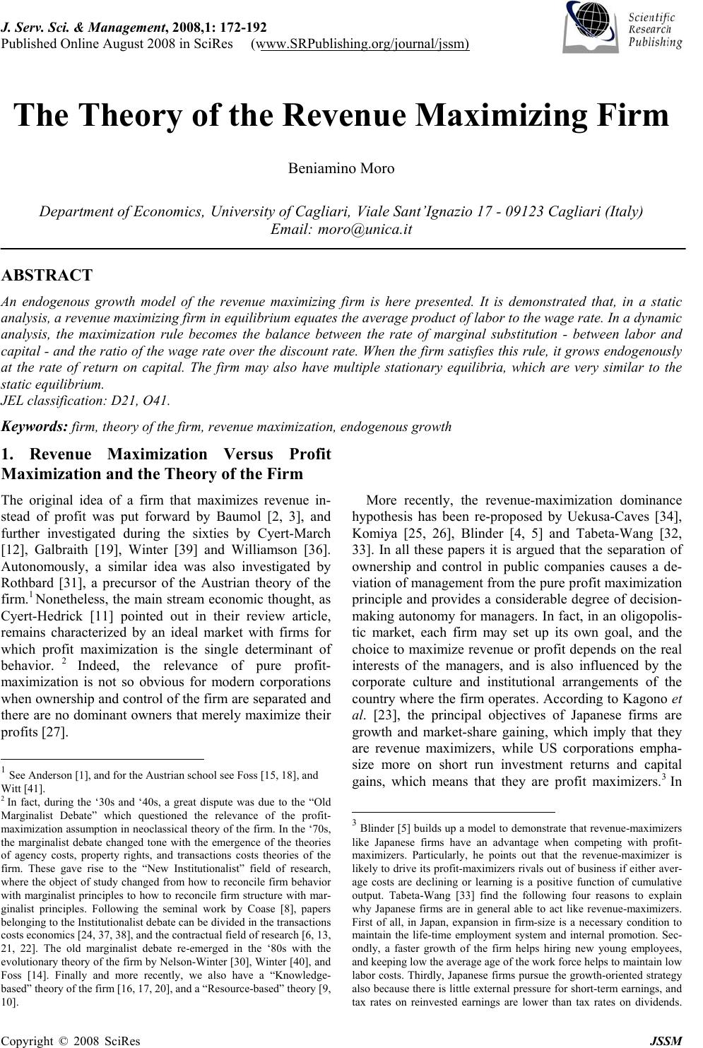J. Serv. Sci. & Management, 2008,1: 172-192
Published Online August 2008 in SciRes (www.SRPublishing.org/journal/jssm)
The Theory of the Revenue Maximizing Firm
Beniamino Moro
Department of Economics, University of Cagliari, Viale Sant’Ignazio 17 - 09123 Cagliari (Italy)
ABSTRACT
An endogenous growth model of the revenue maximizing firm is here presented. It is demonstrated that, in a static
analysis, a revenue maximizing firm in equilibrium equates the average product of labor to the wage rate. In a dynamic
analysis, the maximization rule becomes the balance between the rate of marginal substitution - between labor and
capital - and the ratio of the wage rate over the discount rate. When the firm satisfies this rule, it grows endogenously
at the rate of return on capital. The firm may also have multiple stationary equilibria, which are very similar to the
static equilibrium.
JEL classification: D21, O4 1.
Keywords: firm, theory of the firm, revenue maximization, endogenous growth
1. Revenue Maximization Versus Profit
Maximization and the Theory of the Firm
The original idea of a firm that maximizes revenue in-
stead of profit was put forward by Baumol [2, 3], and
further investigated during the sixties by Cyert-March
[12], Galbraith [19], Winter [39] and Williamson [36].
Autonomously, a similar idea was also investigated by
Rothbard [31], a precursor of the Austrian theory of the
firm.1 Nonetheless, the main stream economic thought, as
Cyert-Hedrick [11] pointed out in their review article,
remains characterized by an ideal market with firms for
which profit maximization is the single determinant of
behavior. 2 Indeed, the relevance of pure profit-
maximization is not so obvious for modern corporations
when ownership and control of the firm are separated and
there are no dominant owners that merely maximize their
profits [27].
1 See Anderson [1], and for the Austrian school see Foss [15, 18], and
Witt [41].
2 In fact, during the ‘30s and ‘40s, a great dispute was due to the “Old
Marginalist Debate” which questioned the relevance of the profit-
maximization assumption in neoclassical theory of the firm. In the ‘70s,
the marginalist debate changed tone with the emergence of the theories
of agency costs, property rights, and transactions costs theories of the
firm. These gave rise to the “New Institutionalist” field of research,
where the object of study changed from how to reconcile firm behavior
with marginalist principles to how to reconcile firm structure with mar-
ginalist principles. Following the seminal work by Coase [8], papers
belonging to the Institutionalist debate can be divided in the transactions
costs economics [24, 37, 38], and the contractual field of research [6, 13,
21, 22]. The old marginalist debate re-emerged in the ‘80s with the
evolutionary theory of the firm by Nelson-Winter [30], Winter [40], and
Foss [14]. Finally and more recently, we also have a “Knowledge-
based” theory of the firm [16, 17, 20], and a “Resource-based” theory [9,
10].
More recently, the revenue-maximization dominance
hypothesis has been re-proposed by Uekusa-Caves [34],
Komiya [25, 26], Blinder [4, 5] and Tabeta-Wang [32,
33]. In all these papers it is argued that the separation of
ownership and control in public companies causes a de-
viation of management from the pure profit maximization
principle and provides a considerable degree of decision-
making autonomy for managers. In fact, in an oligopolis-
tic market, each firm may set up its own goal, and the
choice to maximize revenue or profit depends on the real
interests of the managers, and is also influenced by the
corporate culture and institutional arrangements of the
country where the firm operates. According to Kagono et
al. [23], the principal objectives of Japanese firms are
growth and market-share gaining, which imply that they
are revenue maximizers, while US corporations empha-
size more on short run investment returns and capital
gains, which means that they are profit maximizers.3 In
3 Blinder [5] builds up a model to demonstrate that revenue-maximizers
like Japanese firms have an advantage when competing with profit-
maximizers. Particularly, he points out that the revenue-maximizer is
likely to drive its profit-maximizers rivals out of business if either aver-
age costs are declining or learning is a positive function of cumulative
output. Tabeta-Wang [33] find the following four reasons to explain
why Japanese firms are in general able to act like revenue-maximizers.
First of all, in Japan, expansion in firm-size is a necessary condition to
maintain the life-time employment system and internal promotion. Sec-
ondly, a faster growth of the firm helps hiring new young employees,
and keeping low the average age of the work force helps to maintain low
labor costs. Thirdly, Japanese firms pursue the growth-oriented strategy
also because there is little external pressure for short-term earnings, and
tax rates on reinvested earnings are lower than tax rates on dividends.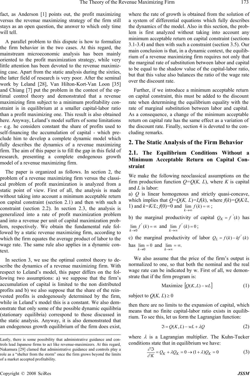

The Theory of the Revenue Maximizing Firm 173
fact, as Anderson [1] points out, the profit maximizing
versus the revenue maximizing strategy of the firm still
stays as an open question, the answer to which only time
will tell.
A parallel problem to this dispute is how to formalize
the firm behavior in the two cases. At this regard, the
mainstream microeconomic analysis has been mainly
oriented to the profit maximization strategy, while very
little attention has been devoted to the revenue maximiz-
ing case. Apart from the static analysis during the sixties,
the latter field of research is very poor. After the seminal
work by Leland [28], Van Hilton-Kort-Van Loon [35]
and Chiang [7] put the problem in the contest of the op-
timal control theory and demonstrated that a revenue
maximizing firm subject to a minimum profitability con-
straint is in equilibrium at a smaller capital-labor ratio
than a profit maximizing one. This result is also obtained
here. Anyway, Leland’s model suffers of some limitations
- e.g. he considers constant the share of profits used to
self-financing the accumulation of capital - which pre-
clude him to develop a complete dynamic model which
fully describes the dynamics of a revenue maximizing
firm. The aim of this paper is to fill the gap in this field of
research, presenting a complete endogenous growth
model of a revenue maximizing firm.
The paper is organized as follows. In section 2, the
problem of a revenue maximizing firm versus the classi-
cal problem of profit maximization is analyzed from a
static point of view. First of all, the analysis is made
without taking into account a minimum acceptable return
on capital constraint (section 2.1) and then with such a
constraint (section 2.2). In section 2.3, the analysis is
generalized into a rate of profit maximization problem
and into a revenue per unit of capital maximization prob-
lem, respectively. We obtain the fundamental rule fol-
lowed by a static revenue maximizing firm, according to
which the firm equates the average product of labor to the
wage rate. The same rule also applies in a dynamic con-
text.
In section 3, we use the optimal control theory to de-
scribe the dynamics of a revenue maximizing firm. With
respect to Leland’s model, this paper differs on the fol-
lowing two assumptions: a) we suppose that the firm’s
accumulation of capital is limited to the non distributed
profits and b) we also suppose that the share of the rein-
vested profits is endogenously determined by the firm,
while in Leland’s model this is a constant. We also dem-
onstrate that only some of the possible dynamic equilibria
(stationary equilibria) correspond to those discussed in
the static analysis. Anyway, it is also demonstrated that
an endogenous growth equilibrium of the firm does exist,
Lastly, there is some possibility that administrative guidance and con-
trols lead Japanese firms to act like revenue-maximizers. At this regard,
Nakamura [29] clamed that administrative guidance and controls play a
role as a “shelter from the storm” once the firm grows beyond the limits
of a market accepted profitability.
where the rate of growth is obtained from the solution of
a system of differential equations which fully describes
the dynamics of the model. Also in this section, the prob-
lem is first analyzed without taking into account any
minimum acceptable return on capital constraint (sections
3.1-3.4) and then with such a constraint (section 3.5). Our
main conclusion is that, in a dynamic context, the equilib-
rium of a revenue maximizing firm requires not only that
the marginal rate of substitution between labor and capital
to be equal to the shadow value of the capital-labor ratio,
but that this value also balances the ratio of the wage rate
over the discount rate.
Further, if we introduce a minimum acceptable return
on capital constraint, this must be added to the discount
rate when determining the equilibrium equality with the
rate of marginal substitution between labor and capital.
As a consequence, a change of the minimum acceptable
return on capital rate has the same effect as a variation of
the discount rate. Finally, section 4 is devoted to the con-
cluding remarks.
2. The Static Analysis of the Firm Behavior
2.1. The Equilibrium Conditions Without a
Minimum Acceptable Return on Capital Con-
straint
We make the following neoclassical assumptions on the
firm production function Q=Q(K, L), where K is capital
and L is labor:
a) Q is linear homogenous and strictly quasi-concave,
which implies that Q=Q(K, L)=Lf(k), where f(k)=Q(K/L,
1) and k=K/L; f(0)=0 and ∞=
∞→ )(lim kf k;
b) the marginal productivity of capital )( 'kfQK= has
∞=
→)( lim' 0kf k and 0)( lim'= ∞→ kf k;
c) the marginal productivity of labor )( )('kkfkfQL−=
has 0lim
0
=
→k and .lim
∞
=
∞→k
We also assume that the price of the firm’s output is
normalized to one, so that both the nominal and the real
wage rate can be indicated by w. First of all, we demon-
strate that if the firm program is:
Maximize
[
]
wLLKQ −),( (1)
subject to Q(K, L)≥0
then there are no limits to the expansion of capital, which
means that no finite capital-labor ratio exists in equilib-
rium. To see this, let us form the Lagrangian function:
QwLLKQ
λ
+
−
=
ℑ
),( (2)
where
λ is a Lagrangian multiplier. The Kuhn-Tucker
conditions state that in equilibrium we have:
0)1(0 =+→=+=
ℑKKK QQQ
K
λλ
∂
∂
(3)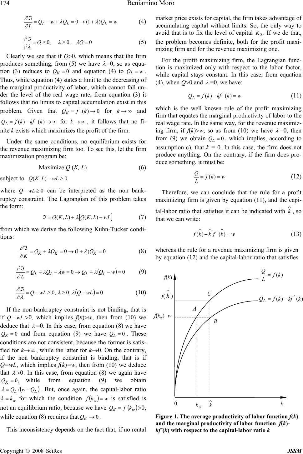

174 Beniamino Moro
wQQwQ
LLLL =+→=+−=
ℑ)1(0
λλ
∂
∂
(4)
0,0,0 =≥≥=
ℑQQ
λλ
λ∂
∂
(5)
Clearly we see that if Q>0, which means that the firm
produces something, from (5) we have λ =0, so as equa-
tion (3) reduces to 0=
K
Q and equation (4) to wQL
=
.
Thus, while equation (4) states a limit to the decreasing of
the marginal productivity of labor, which cannot fall un-
der the level of the real wage rate, from equation (3) it
follows that no limits to capital accumulation exist in this
problem. Given that 0)(
'→= kfQK for
∞
→k and
∞→−= )( )('kkfkfQL for ∞→k, it follows that no fi-
nite k exists which maximizes the profit of the firm.
Under the same conditions, no equilibrium exists for
the revenue maximizing firm too. To see this, let the firm
maximization program be:
Maximize Q (K, L) (6)
subject to 0),( ≥− wLLKQ
where 0≥−wLQ can be interpreted as the non bank-
ruptcy constraint. The Lagrangian of this problem takes
the form:
[
] wLLKQLKQ −+=ℑ),(),(
λ
(7)
from which we derive the following Kuhn-Tucker condi-
tions:
0)1(0 =+→=+=
ℑKKK QQQ
K
λλ
∂
∂
(8)
() 00 =−+→=−+=
ℑwQQwQQ
LLLLL
λλλ
∂
∂
(9)
() 0,0,0 =−≥≥−=
ℑwLQwLQ
λλ
λ∂
∂
(10)
If the non bankruptcy constraint is not binding, that is
if wLQ −>0, which implies f(k)>w, then from (10) we
deduce that
λ
=0. In this case, from equation (8) we have
0=
K
Q and from equation (9) we have 0=
L
Q. These
conditions are not consistent, because the former is satis-
fied for k→∞, while the latter for k→0. On the contrary,
if the non bankruptcy constraint is binding, that is if
Q=wL, which implies f(k)=w, then from (10) we deduce
that
λ
>0. In this case, from equation (8) we again have
,0=
K
Qwhile from equation (9) we obtain
()
LL QwQ −= /
λ
. But, once again, the capital-labor ratio
w
kk = for which the condition
()
wkfw= is satisfied is
not an equilibrium ratio, because we have
(
)
wK kfQ =>0,
while equation (8) requires that0→
K
Q.
This inconsistency depends on the fact that, if no rental
market price exists for capital, the firm takes advantage of
accumulating capital without limits. So, the only way to
avoid that is to fix the level of capital 0
K. If we do that,
the problem becomes definite, both for the profit maxi-
mizing firm and for the revenue maximizing one.
For the profit maximizing firm, the Lagrangian func-
tion is maximized only with respect to the labor factor,
while capital stays constant. In this case, from equation
(4), when Q>0 and
λ
=0, we have:
wkkfkfQL=−= )( )(' (11)
which is the well known rule of the profit maximizing
firm that equates the marginal productivity of labor to the
real wage rate. In the same way, for the revenue maximiz-
ing firm, if f(k)>w, so as from (10) we have
λ
=0, then
from (9) we obtain 0=
L
Q, which implies, according to
assumption c), that k = 0. In this case, the firm does not
produce anything. On the contrary, if the firm does pro-
duce something, it must be:
wkf
L
Q== )( (12)
Therefore, we can conclude that the rule for a profit
maximizing firm is given by equation (11), and the capi-
tal-labor ratio that satisfies it can be indicated with
∧
k, so
that we can write:
wkfkkf =− ∧∧∧ )( )(' (13)
whereas the rule for a revenue maximizing firm is given
by equation (12) and the capital-labor ratio that satisfies
Figure 1. The average productivity of labor function f(k)
and the marginal productivity of labor function f(k)-
kf’(k) with respect to the capital-labor ratio k
k
∧
k
w
k
0
)(kf
L
Q=
B
C
f
(kw)=w
f
(
k
∧
)
f
(k)
)( )('kkfkfQL−=
A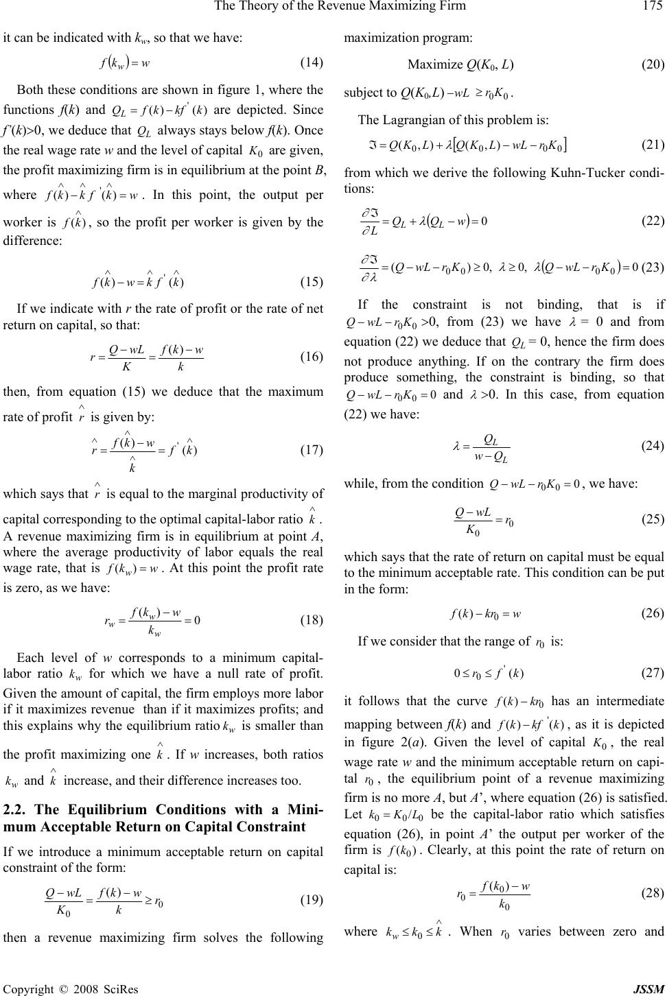

The Theory of the Revenue Maximizing Firm 175
it can be indicated with kw, so that we have:
() wkfw= (14)
Both these conditions are shown in figure 1, where the
functions f(k) and )( )('kkfkfQL−= are depicted. Since
f’(k)>0, we deduce that L
Q always stays below f(k). Once
the real wage rate w and the level of capital 0 K are given,
the profit maximizing firm is in equilibrium at the point B,
where wkfkkf =− ∧∧∧ )( )('. In this point, the output per
worker is )(
∧
kf , so the profit per worker is given by the
difference:
)( )('∧∧∧ =− kfkwkf (15)
If we indicate with r the rate of profit or the rate of net
return on capital, so that:
k
wkf
K
wLQ
r− =
−
=)( (16)
then, from equation (15) we deduce that the maximum
rate of profit
∧
r
is given by:
)(
)( '∧
∧
∧
∧=
−
=kf
k
wkf
r (17)
which says that
∧
r
is equal to the marginal productivity of
capital corresponding to the optimal capital-labor ratio
∧
k.
A revenue maximizing firm is in equilibrium at point A,
where the average productivity of labor equals the real
wage rate, that is wkf w=)( . At this point the profit rate
is zero, as we have:
0
)( = −
=
w
w
wk
wkf
r (18)
Each level of w corresponds to a minimum capital-
labor ratio w k for which we have a null rate of profit.
Given the amount of capital, the firm employs more labor
if it maximizes revenue than if it maximizes profits; and
this explains why the equilibrium ratiow
k is smaller than
the profit maximizing one
∧
k. If w increases, both ratios
w
k and
∧
k increase, and their difference increases too.
2.2. The Equilibrium Conditions with a Mini-
mum Acceptable Return on Capital Constraint
If we introduce a minimum acceptable return on capital
constraint of the form:
0
0
)( r
k
wkf
K
wLQ ≥ −
=
− (19)
then a revenue maximizing firm solves the following
maximization program:
Maximize Q(K0, L) (20)
subject to Q(K0,L)wL
−
00Kr≥.
The Lagrangian of this problem is:
[
]
0000 ),(),( KrwLLKQLKQ −−+=ℑ
λ (21)
from which we derive the following Kuhn-Tucker condi-
tions:
() 0=−+=
ℑwQQ
LLL
λ
∂
∂
(22)
()
0,0,0)( 0000=−−≥≥−−=
ℑKrwLQKrwLQ
λλ
λ∂
∂
(23)
If the constraint is not binding, that is if
00KrwLQ
−
−
>0, from (23) we have
λ
= 0 and from
equation (22) we deduce that L Q= 0, hence the firm does
not produce anything. If on the contrary the firm does
produce something, the constraint is binding, so that
0
00 =−−KrwLQ and
λ
>0. In this case, from equation
(22) we have:
L
L
Qw
Q
−
=
λ (24)
while, from the condition 0
00 =−−KrwLQ, we have:
0
0
r
K
wLQ= − (25)
which says that the rate of return on capital must be equal
to the minimum acceptable rate. This condition can be put
in the form:
wkrkf =− 0 )( (26)
If we consider that the range of 0 r is:
)( 0'
0kfr≤≤ (27)
it follows that the curve 0 )( krkf − has an intermediate
mapping between f(k) and )( )('kkfkf −, as it is depicted
in figure 2(a). Given the level of capital 0 K, the real
wage rate w and the minimum acceptable return on capi-
tal 0
r, the equilibrium point of a revenue maximizing
firm is no more A, but A’, where equation (26) is satisfied.
Let 000/LKk = be the capital-labor ratio which satisfies
equation (26), in point A’ the output per worker of the
firm is )( 0 kf . Clearly, at this point the rate of return on
capital is:
0
0
0
)(
k
wkf
r− = (28)
where
∧
≤≤ kkkw0. When 0 r varies between zero and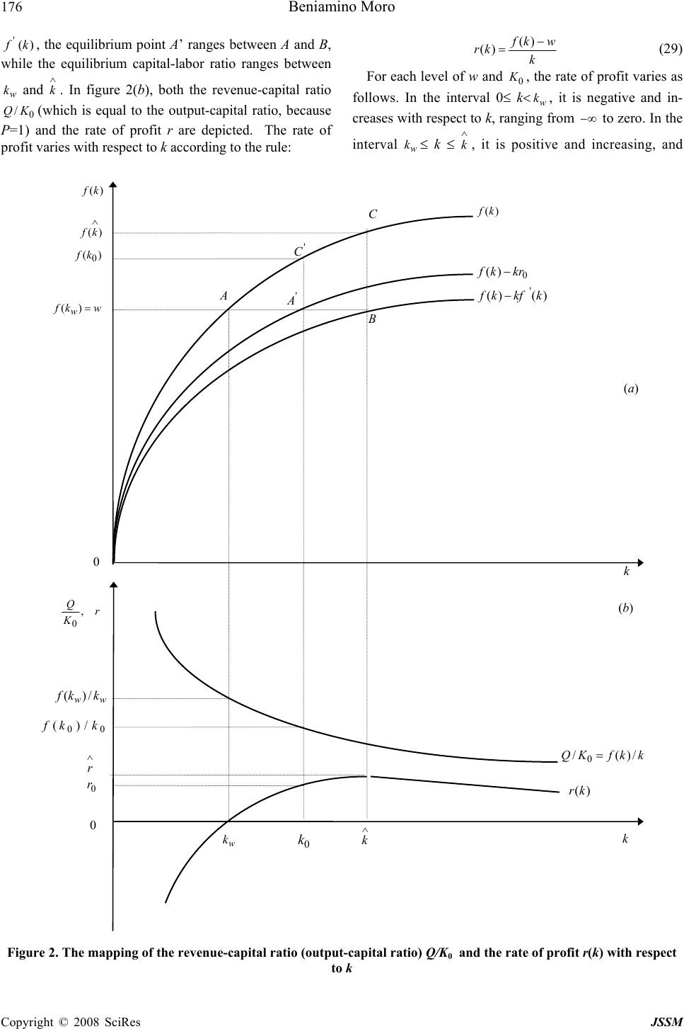

176 Beniamino Moro
)(
'kf , the equilibrium point A’ ranges between A and B,
while the equilibrium capital-labor ratio ranges between
w
k and
∧
k. In figure 2(b), both the revenue-capital ratio
0
/KQ (which is equal to the output-capital ratio, because
P=1) and the rate of profit r are depicted. The rate of
profit varies with respect to k according to the rule:
k
wkf
kr−
=)(
)( (29)
For each level of w and 0 K, the rate of profit varies as
follows. In the interval 0≤ k<w
k, it is negative and in-
creases with respect to k, ranging from −∞ to zero. In the
interval w k≤ k ≤ ∧ k, it is positive and increasing, and
Figure 2. The mapping of the revenue-capital ratio (output-capital ratio) Q/K0 and the rate of profit r(k) with respect
to k
(b)
0
(a)
k
w
k
A
wkf w=)(
)(0 kf
)(
∧
kf
)(kf
0
k∧
kk
kkfKQ /)(/ 0=
)(kr
r
K
Q,
0
ww kkf /)(
00/)( kkf
∧
r
0
r
0
'
C
'
A
B
C)(kf
0
)( krkf
−
)( )('kkfkf −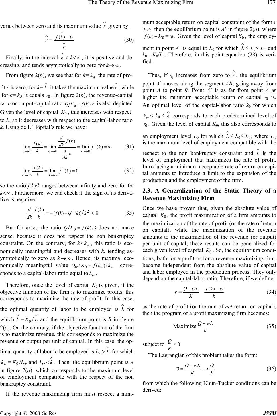

The Theory of the Revenue Maximizing Firm 177
varies between zero and its maximum value
∧
r
given by:
∧
r
= ∧
∧−
k
wkf )( (30)
Finally, in the interval ∧
k< k<∞, it is positive and de-
creasing, and tends asymptotically to zero for k→
∞
.
From figure 2(b), we see that for k= w
k the rate of pro-
fit r is zero, for k= ∧
k it takes the maximum value∧
r
, while
for k= 0
k it equals 0
r. In figure 2(b), the revenue-capital
ratio or output-capital ratio kkfKQ/)(
0= is also depicted.
Given the level of capital 0
K, this increases with respect
to L, so it decreases with respect to the capital-labor ratio
k. Using de L’Hôpital’s rule we have:
∞=== →→→ )( lim
)(
lim
)(
lim '
000 kf
k
dk
d
kf
dk
d
k
kf
kkk (31)
0)( lim
)(
lim '== ∞→∞→ kf
k
kf
kk (32)
so the ratio f(k)/k ranges between infinity and zero for 0<
k<∞. Furthermore, we can check if the sign of its deriva-
tive is negative:
k
kf
dk
d)( =2' )]( )([kkkfkf −− < 0 (33)
But for k<w k the ratio kkfKQ/)(
0=does not make
sense, because it does not respect the non bankruptcy
constraint. On the contrary, for k≥w
k, this ratio is eco-
nomically meaningful and decreases with k, tending as-
ymptotically to zero as k∞→ . Hence, its maximal eco-
nomically meaningful value www kkfKQ /)(/ 0= corre-
sponds to a capital-labor ratio equal tow k.
Therefore, once the level of capital K0 is given, if the
objective function of the firm is to maximize profits, this
corresponds to maximize the rate of profit. In this case,
the optimal quantity of labor to be employed is
∧
L
for
which
∧
k=0 K/
∧
L
and the equilibrium point is B in figure
2(a). On the contrary, if the objective function of the firm
is to maximize revenue, this corresponds to maximize the
revenue or output per unit of capital. In this case, the op-
timal quantity of labor to be employed is Lw >∧
L
for which
w
k=0 K/Lw and w k<∧ k. Then, the equilibrium point is A
in figure 2(a), which corresponds to the maximum level
of employment compatible with the respect of the non
bankruptcy constraint.
If the revenue maximizing firm must respect a mini-
mum acceptable return on capital constraint of the form r
≥ r0, then the equilibrium point is A’ in figure 2(a), where
0
)( krkf
−
= w. Given the level of capital0 K, the employ-
ment in point A’ is equal to L0 for which
∧
L
≤ L0≤ Lw and
k0= K0/L0. Therefore, in this point equation (28) is veri-
fied.
Thus, if 0 r increases from zero to
∧
r
, the equilibrium
point A’ moves along the segment AB, going away from
point A to point B. Point A’ is as far from point A as
higher the minimum acceptable return on capital 0
r is.
An optimal level of the capital-labor ratio k0 for which
w
k≤ k0 ≤ ∧ k corresponds to each predetermined level of
0
r. Given the level of capital K0, this also corresponds to
an employment level L0 for which
∧
L
≤ L0≤ Lw, where Lw
is the maximum level of employment compatible with the
respect to the non bankruptcy constraint and
∧
L
is the
level of employment that maximizes the rate of profit.
Introducing a minimum acceptable rate of return on capi-
tal amounts to introduce a limit to the expansion of the
production and the employment of the firm.
2.3. A Generalization of the Static Theory of a
Revenue Maximizing Firm
Once we have proven that, given the absolute value of
capital 0
K, the profit maximization of a firm amounts to
the maximization of the rate of profit (or the rate of return
on capital), while the maximization of the revenue
amounts to the maximization of the revenue (or output)
per unit of capital, these results can be generalized for
each given level of capital 0
K. So, the equilibrium condi-
tions, both for a profit or for a revenue maximizing firm,
become independent from the absolute value of capital
and labor employed in the production process. They only
depend on the capital-labor ratio. Therefore, if we define:
r =k
wkf
K
wLQ −
=
−)( (34)
as the rate of profit (or the rate of net return on capital),
then the program of a profit maximizing firm becomes:
Maximize K
wLQ − (35)
subject to 0≥
K
Q
The Lagrangian of this problem takes the form:
K
Q
K
wLQ
λ +
−
=ℑ (36)
from which the following Khun-Tucker conditions can be
derived:

178 Beniamino Moro
22
)(
K
QKQ
K
wLQKQ
KKK
λλ
∂
∂ −
+
−−
=
ℑ = 0 (37)
0=+
−
=
ℑ
K
Q
K
wQ
LLL
λ
∂
∂
(38)
0,0,0 =≥≥=
ℑ
K
Q
K
Q
λλ
λ∂
∂
(39)
Equations (37) and (38) can also be stated in the form:
(1+
λ
)
[]
wLKQQ K=− (40)
(1+
λ
)L Q=w (41)
If the firm produces, then Q/K>0 and from equation
(39) we deduce that λ =0, thus equations (40) and (41)
take the form:
Q
− KK Q= wL → )( )('kkfkf−= w (42)
L
Q= )( )('kkfkf −= w (43)
These two equations state the same maximization rule,
corresponding to the equality of the marginal productivity
of labor to the real wage rate. This again re-asserts that
the equilibrium capital-labor ratio for a profit maximizing
firm is
∧
k.
Likewise, the program of a revenue maximizing firm
becomes:
Maximize K
Q (44)
subject to 0≥
−
K
wLQ
where the firm respects a non bankruptcy constraint. To
solve this problem, let us form the Lagrangian function:
()
K
wLQ
K
Q−
+=ℑ
λ
(45)
from which the following Kuhn-Tucker conditions can be
derived:
[]
0
)(
22=
−−
+
−
=
ℑ
K
wLQKQ
K
QKQ
KKK
λ
∂
∂
(46)
0
)( = −
+=
ℑ
K
wQ
K
Q
LLL
λ
∂
∂
(47)
0
)(
,0,0 =
−
≥≥
−
=
ℑ
K
wLQ
K
wLQ λ
λ
λ∂
∂
(48)
Equations (46) and (47) can be put in the form:
(1+
λ
) (Q − KK Q)= λ wL (49)
(1+
λ
)L Q=
λ
w (50)
respectively. If the non bankruptcy constraint is not bind-
ing, that is if Q
− wL>0, then from (48) we deduce
λ
=0. In
this case, from equation (50) we have L Q=0, which im-
plies:
L
Q=)( )('kkfkf −=0 (51)
or:
f(k)= )(
'kkf (52)
This last equation is satisfied only for k=0, that is,
when the firm does not produce anything. Analogously,
for
λ
=0, also equation (49) leads to the same conclusion.
In fact, if
λ
=0, then Q=KK
Q, and dividing by L we ob-
tain (52). It follows that, if the firm produces, the non
bankruptcy constraint must be binding, which implies:
Q − wL=0 → f(k)=w (53)
In this case, from (48) we deduce that
λ
>0 and the
value of
λ
can be determined either from (49) or (50).
Using the latter, we have:
(1+
λ
)[ )( )('kkfkf −]=
λ
f(k) (54)
The same result is obtained from (49) dividing by L.
From (54) we have:
K
L
kQ
Q
kkf
kkfkf = −
=
)(
)( )(
'
'
λ (55)
which defines the equilibrium value of
λ
. Equation (55)
can also be put in the form:
KL
MRS /=k
Q
Q
K
L
λ = (56)
where KL MRS / stays for the marginal rate of substitution
between labor and capital. If we interpret
λ as the shadow
price of capital, then (56) means that in equilibrium the
marginal rate of substitution must equal the shadow value
of per capita capital. As we shall see later, this rule also
applies in a dynamic analysis. Because equations (53) and
(56) are satisfied for k= w
k, it is confirmed that the equi-
librium capital-labor ratio for a revenue maximizing firm
is w k, that is the value of k which guaranties the equality
between the average productivity of labor and the real
wage rate.
Finally, if the firm must satisfy a minimum return on
capital constraint, the maximization program is as follows:
Maximize K
Q (57)
subject to 0 r
K
wLQ ≥ −
where r0 is the minimum acceptable rate of return on
capital. The Lagrangian of this problem is:
⎥
⎦
⎤
⎢
⎣
⎡−
−
+=ℑ0
r
K
wLQ
K
Q
λ (58)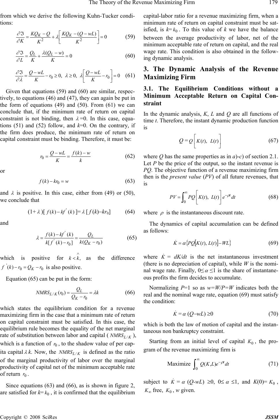

The Theory of the Revenue Maximizing Firm 179
from which we derive the following Kuhn-Tucker condi-
tions:
0
)(
22 =
⎥
⎦
⎤
⎢
⎣
⎡−−
+
−
=
ℑ
K
wLQKQ
K
QKQ
KKK
λ
∂
∂
(59)
0
)( = −
+=
ℑ
K
wQ
K
Q
LLL
λ
∂
∂
(60)
0,0,0 00 =
⎥
⎦
⎤
⎢
⎣
⎡−
−
≥≥−
−
=
ℑr
K
wLQ
r
K
wLQ
λλ
λ∂
∂
(61)
Given that equations (59) and (60) are similar, respec-
tively, to equations (46) and (47), they can again be put in
the form of equations (49) and (50). From (61) we can
conclude that, if the minimum rate of return on capital
constraint is not binding, then
λ
=0. In this case, equa-
tions (51) and (52) follow, and k=0. On the contrary, if
the firm does produce, the minimum rate of return on
capital constraint must be binding. Therefore, it must be:
k
wkf
K
wLQ
r− =
−
=)(
0 (62)
or
wkrkf =− 0 )( (63)
and
λ
is positive. In this case, either from (49) or (50),
we conclude that
(1+
λ
)[ )( )('kkfkf −]=
λ
[ f (k)−kr0] (64)
and
)(
])( [
)( )(
0
0
'
'
rQk
Q
rkfk
kkfkf
K
L
−
=
−
−
= λ (65)
which is positive for,
∧
<kk as the difference
00
')( rQrkfK−=− is also positive.
Equation (65) can be put in the form:
k
rQ
Q
rNMRS K
L
KL
λ =
−
=
0
0/ )( (66)
which states the equilibrium condition for a revenue
maximizing firm in the case that a minimum rate of return
on capital constraint must be satisfied. In this case, the
equilibrium rule becomes the equality of the net marginal
rate of substitution between labor and capital (KL
NMRS /),
which is a function of 0
r, to the shadow value of per cap-
ita capital
λ
k. Now, the KL NMRS / is defined as the ratio
of the marginal productivity of labor over the marginal
productivity of capital net of the minimum acceptable rate
of return 0 r.
Since equations (63) and (66), as is shown in figure 2,
are satisfied for k=0
k, it is confirmed that the equilibrium
capital-labor ratio for a revenue maximizing firm, when a
minimum rate of return on capital constraint must be sat-
isfied, is k=0
k. To this value of k we have the balance
between the average productivity of labor, net of the
minimum acceptable rate of return on capital, and the real
wage rate. This condition is also obtained in the follow-
ing dynamic analysis.
3. The Dynamic Analysis of the Revenue
Maximizing Firm
3.1. The Equilibrium Conditions without a
Minimum Acceptable Return on Capital Con-
straint
In the dynamic analysis, K, L and Q are all functions of
time t. Therefore, the instant dynamic production function
is
Q =⎥
⎦
⎤
⎢
⎣
⎡)(),(tLtKQ (67)
where Q has the same properties as in a)-c) of section 2.1.
Let P be the price of the output, so the instant revenue is
PQ. The objective function of a revenue maximizing firm
then is the present value (PV) of all future revenues, that
is
dtetLtKPQPV t
ρ −
∞
∫⎥
⎦
⎤
⎢
⎣
⎡
=
0
)(),( (68)
where
ρ
is the instantaneous discount rate.
The dynamics of capital accumulation can be defined
as follows:
[] {} WLtLtKPQK −= )(),( α
& (69)
where
K
&= dK/dt is the net instantaneous investment
(there is no depreciation of capital), while W is the nomi-
nal wage rate. Finally, 0≤
α
≤1 is the share of instantane-
ous profits the firm decides to accumulate.
Normalizing P=1 so as w=W/P=W indicates both the
real and the nominal wage rate, equation (69) must satisfy
the condition:
K
&=
α
(Q − wL) ≥0 (70)
which is both the law of motion of capital and the instan-
taneous non bankruptcy constraint.
Starting from an initial level of capital 0
K, the pro-
gram of the revenue maximizing firm is
Maximize ∫∞−
0
),( dteLKQt
ρ
(71)
subject to
K
&=
α
(Q-wL) ≥0, 0≤
α
≤1, and K(0)= 0 K,
∞
Kfree, 0 K, w given.

180 Beniamino Moro
In this problem, K is the state variable while L is a con-
trol variable. What about
α
, which is the share of instan-
taneous profits the firm decides to accumulate?4 In fact,
we can suppose that the firm can decide in each instant of
time to accelerate the speed of capital accumulation by
increasing the value of
α
. We have the maximum speed
if
α
=1, while there is no capital accumulation if
α
=0. In
the latter case, all profits are distributed to the stockhold-
ers. Hence, it is obvious to consider
α
as a second con-
trol variable of the problem.
To solve the program (71), let us indicate with C
H the
current value Hamiltonian:
)(),(wLQLKQHC−+=
λα
(72)
where
λ
is a dynamic Lagrangian multiplier. Further-
more, as the costate variable is strictly adherent to the
state variable K,
λ
can also be interpreted as the shadow
price of capital.
Because the Hamiltonian is linear with respect to,
α
the
maximization rule 0/
=
α
∂
∂
C
H does not apply in this
case. Instead, we have a maximum in one of the extreme
values of the
α
interval [0, 1]. Moreover, since
λ
is
positive, as we will see later, C H is maximized for
α
=1
if Q − wL>0, while, for Q − wL=0,
α
is indeterminate.
Furthermore, since Q is a strictly quasi-concave function,
the Hamiltonian C H is a concave function of K and L. So,
the following conditions of the maximum principle are
necessary and sufficient for the solution of the program
(71):
0)(=−+= wQQ
L
HLL
C
λα
∂
∂
(73)
)( wLQ
H
KC−== α
λ∂
∂
& (74)
ρλλαρλ
∂
∂
λ +−−=+−=KK
CQQ
K
H
& (75)
0lim,0lim == −
∞→
−
∞→
t
t
t
C
teeH
ρρ
λ (76)
Condition (73) guarantees the employment of the labor
factor is optimized along the time path L(t). If the firm
does make profits, Q − wL>0 and
α
=1, and from condi-
tion (73) we obtain:
)]( )([
)( )(
'
'
kkfkfw
kkfkf
Qw
Q
L
L
−−
−
=
−
= λ (77)
This is the dynamic optimization rule the firm follows
4 In Leland’s model [28],
α
is an exogenous parameter on which the
firm exerts no influence. This assumption is not realistic and, at the same
time, it contributes to limit Leland’s analysis.
in the employment of the labor factor, which corresponds
to condition (9) and conditions (22) or (24) from a static
point of view. This rule requires that the firm must bal-
ance the ratio of the marginal productivity of labor over
the wage rate, net of the same marginal productivity of
labor, to the shadow price of capital along the entire time
path of the costate variable
λ
.
Condition (74) again represents the dynamics of capital,
while condition (75) is the equation of motion of the co-
state variable
λ
. Equations (74) and (75) together form
the Hamiltonian or canonical system.
Finally, equations (76) are the transversality conditions.
The first one requires the limit of the present-value Ham-
iltonian vanishes as t→
∞
. The second one requires the
shadow price of capital in discounted value vanishes as
t→
∞
. Since the term t e
ρ −→0 as t→∞, both these trans-
versality conditions are satisfied for finite values of HC ≠0,
and
λ
≠0. This will be demonstrated in section 3.4.
Condition (74), dividing by L and remembering that
α
=1, can be put in the form:
wkf
L
K−= )(
&
(78)
Since from the definition of k=K/L we have K=kL, and
K
&=k
&L+k
L
&, dividing by L and substituting we obtain:
wkf
L
L
kk
L
K−=+= )(
&
&
&
(79)
and finally:
L
L
kwkfk&
&−−= )( (80)
Given the real wage rate w, equation (80) describes the
dynamics of the capital-labor ratio as a function of the
rate of growth of employment LL/
&. Analogously, from
condition (75), setting
α
=1, we obtain:
)( )]( ['' kfkf −
−
=
ρ
λ
λ
& (81)
which describes the dynamics of
λ
, given
ρ
, as a func-
tion of the capital-labor ratio.
Conditions (77), (80) and (81), taken together, form a
system of three equations, two of which are differential
equations, in three unknowns, given by k,
λ
and LL/
&.
These equations fully describe the dynamics of a revenue
maximizing firm. Given the real wage rate w and the dis-
count rate
ρ
, we can find a steady state equilibrium for
0== λ
&
&
k. This equilibrium is characterized by a time
constant value of the triple (k,
λ
, LL/
&). Furthermore, our
system can be decomposed into two sub-systems: the first
one made up by equations (77) and (81), where the vari-
able LL/
& does not appear, and the second one corre-

The Theory of the Revenue Maximizing Firm 181
sponding to equation (80) alone, which is the only equa-
tion where the employment rate of growth LL/
& is pre-
sent. So, the first subsystem made up by equations (77)
and (81) can be solved autonomously, and its solution
gives, for λ
&= 0, the steady state values of k and
λ
. Sub-
stituting the equilibrium value of k in equation (80) and
setting k
&= 0, the second subsystem yields the equilib-
rium growth rate of employmentLL/
&.
Now, let us concentrate, first of all, on the subsystem
made up by equations (77) and (81), which can be de-
picted in a phase diagram on the plane k,
λ
. To construct
this, we must pay attention to equation (77). Like in the
static analysis, let us indicate with
∧
k the capital-labor
ratio which satisfies the equality between the marginal
productivity of labor and the real wage rate, that is
L
Q=)( )('∧∧∧−kfkkf =w; and let us indicate with w k the
capital-labor ratio which satisfies the equality between the
average productivity of labor and the real wage rate, that
is wkf w=)( . From equation (77), since L Q→0 as k→0,
whereas the ratio QL /(w − QL) → ∞ as (w − QL) →0 and
k→∧ k, we deduce that
λ
is an increasing function of k,
which goes from zero to infinity as k goes from zero to
∧
k.
Furthermore, we can find that the sign of the derivative of
λ
with respect to k is positive. To find this, let us write
equation (77) in the implicit form:
0])( )([)( )(),('' =−−+−= wkkfkfkkfkfkGw λλ (82)
where w
G is the implicit function existing between k and
λ
. The sub-index w in G means that this function is de-
fined for any given w. Differentiating (82), we have:
wkkfkf
kkf
G
kG
kd
d
w
w
−−
+
=−=
)( )(
)( )1(
/
/
'
"
λ
λ∂∂
∂∂ λ
> 0 (83)
which is positive because for
∧
<kk we have w
>)( )('kkfkf − and )( "kf < 0.
Figure 3. The mapping of the function Gw(k, λ )
However, equation (77) is not economically meaning-
ful for 0≤ k<w k, because in this range the non bankruptcy
constraint is not satisfied. Anyway, for k =w k, the firm
does not make profits, so we have Q − wL=0 and
α
is
indeterminate in the open range
α
[ ) 1 ,0∈. In this case,
from (73) we obtain:
)]( )([
)( )(
][ '
'
www
www
L
L
kfkkfw
kfkkf
Qw
Q
+−
−
=
−
=
α
α
λ (84)
where
λ
is defined with respect to
α
for k =w k. The
mapping of the function 0),( =
λ
kGw is depicted in figure 3.
The part of this function that has an economic meaning
belongs to the range [w k,
∧
k); for k =w k, the function
0),(
=
λ
kGw becomes a truncated vertical line, where the
truncation point A is given by:
)]( )([
)( )(
lim '
'
kkfkfw
kkfkf
w
kk
A−−
−
=→
λ (85)
where the limit is calculated as k→w k from the right. For
w
k<k<∧ k, instead, the curve 0),( =
λ
kGw is defined by
the expression (77).
Since the equilibrium condition the firm must respect
in employing labor is satisfied only along the curve
0),(
=
λ
kGw, it follows that the dynamics of the firm can
be fully described only by a point of this curve belonging
to the range [w k,
∧
k). To find this point, we need to take
into account condition (81), which describes the dynam-
ics of the shadow price of capital
λ
.
The static analysis has suggested that a profit maximiz-
ing firm is in equilibrium in
∧
k, while a revenue maximiz-
ing firm is in equilibrium in w k. Furthermore, if a reve-
nue maximizing firm must also respect a minimum ac
Figure 4. The mapping of the λ
&= 0 curve
k
∧
k
w
k
0
A
λ
λ
0),(= λ kGw
A
λ
Max
λ
B
λ
0
k
+
k
k
w
B
0=
λ
&
'
B

182 Beniamino Moro
ceptable return on capital constraint, its equilibrium point
is intermediate between w
k and
∧
k. We are led to an
analogous conclusion in a dynamic context too, but with a
fundamental specification. As long as the firm grows, the
dynamic equilibrium point is intermediate between w
k
and ∧ k. Once the firm stops growing, the stationary equi-
librium of a revenue maximizing firm is the same as the
static one and corresponds to a capital-labor ratio equal
to w k.
When a revenue maximizing firm must also respect a
minimum acceptable return on capital constraint in a dy-
namic context, we have two cases. If the constraint is not
binding, in the equilibrium point the firm grows at a rate
which is smaller than the rate of profit. Otherwise, if the
constraint is binding, the firm does not grow any more. In
the latter case, all profits that the firm realizes are distrib-
uted to the stockholders to satisfy the minimum accept-
able return on capital constraint, and nothing remains to
the firm for self-financing and capital accumulation. The
equilibrium point k0, being
∧
≤≤ kkkw0, is the capital-
labor ratio to which it corresponds a rate of profit exactly
equal to the minimum return on capital rate 0
r. Obviously,
also in this case the firm rate of growth is zero. We dem-
onstrate all this in the following sections.
3.2. The Equilibrium Capital-labor Ratio
As previously seen, the dynamics of the costate variable
λ
is given by equation (81). First we need to map in a
phase diagram the stationary points of
λ
, given by:
0)( )]( ['' =−−=kfkf αρλλ
& (86)
from which we obtain:
)(
)(
)0( '
'
kf
kf
αρ
λλ
−
==
& (87)
If the firm makes profits, Q − wL>0 and
α
=1. In this
case, equation (87) reduces to:
)(
)(
)0( '
'
kf
kf
−
==
ρ
λλ
& (88)
which describes the stationary points of the shadow price
of capital
λ
with respect to the capital-labor ratio k. The
map of this curve, from now on defined as the λ
&= 0
curve, which is depicted in figure 4, depends on the value
of
ρ
. For
ρ
<)(
'kf , the curve
λ
&= 0 gives negative val-
ues of
λ
, which are not economically meaningful. There-
fore it must be
ρ
≥)(
'kf in order to have significant eco-
nomic values of
λ
.
Let k+ be the level of k which satisfies the equation
)(
'+
−kf ρ = 0, so if k→ k+ from the right, then we have
λ
→
∞
. Since )( kf decreases with k, for k > k+ we have
)(
'kf−
ρ > 0, and
λ
>0, so we have positive values of the
shadow price of capital. Furthermore, always for values
of k> k+, differentiating equation (86), we have:
)(
)( )1(
/
/
'
"
kf
kfk
dk
d
−
+
=−=
ρ
λ
λ∂λ∂
∂λ∂λ
&
&< 0 (89)
The sign of this expression is negative because the de-
nominator is positive, while )( "kf < 0. As k→ k+ from
the right, )]( ['kf− ρ →0, so ∞−→kdd /
λ
. This means that
the curve λ
&=0 is asymptotic as k→ k+
from the right,
decreases as k increases and becomes zero as k→
∞
, be-
ing .0)( lim'=
∞→ kf k
By definition, the value of k+ depends on the discount
rate
ρ
. For sufficiently high values of
ρ
, we find that k+
has an intermediate value between zero andw k. In this
case, the curve λ
&= 0 is economically meaningful only for
k ≥w k, that is to say only for those values of k for which
the non bankruptcy constraint is satisfied. For k >w k, the
curve λ
&= 0 is defined by equation (88), while for k =w
k
the curve is defined by equation (87) with a value of
α
which varies in the open interval 0≤
α
<1. In the latter
case, the stationary values of
λ
are given by:
)(
)(
)0( '
'
w
w
kf
kf
αρ
λλ
−
==
& (90)
As
α
varies, equation (90) describes the segment BB’,
whose extreme value at B’ (obtained for
α
= 0) is
ρ
λ
)(
'w
Max kf
= (91)
while in point B the stationary value of
λ
is given by:
)(
)(
)(
)(
lim '
'
'
'
w
w
kk
Bkf
kf
kf
kf
w−
=
−
=→
ρρ
λ (92)
where the limit is calculated as k→w k from the right.
Overlapping the two curves 0),(=
λ
kGw and λ
&= 0 on the
same graph, we can depict the phase diagram of our
model. We can have many cases, depending on the rela-
tive location of the points A, B e B’. For B
λ
>A
λ
, where
A
λ
is defined by equation (85), we have the situation
depicted in figure 5. In this case, the dynamic equilibrium
of a revenue maximizing firm may occur at two points of
the capital-labor ratio, corresponding respectively to k
and w k. However, the only dynamic equilibrium is point
E, to which an endogenous growth of the firm corre-
sponds, which is defined by the pair of values),(
−−
λ k.

The Theory of the Revenue Maximizing Firm 183
Figure 5. The phase diagram for 0 < k+< kw
At this point, the dynamic equilibrium of a revenue
maximizing firm is characterized by the stationarity of
both the capital-labor ratio at the level k and the shadow
price of capital at the level
−
λ . The equilibrium value of
the capital-labor ratio k can be found taking the equa-
tions (77) and (88) as a system of simultaneous equations,
whose solution gives:
)(
)(
)( )(
)( )(
'
'
'
'
kf
kf
kkfkfw
kkfkf
−
=
+−
−
ρ
(93)
while the equilibrium value of the capital shadow price
λ is given by:
)]( )([
)( )(
)(
)(
'
'
'
'
kfkkfw
kfkkf
kf
kf
−−
−
=
−
=
ρ
λ (94)
From equation (93), rearranging we obtain:
ρ
w
kf
kkfkf = −
)(
)( )(
'
'
(95)
which can be expressed in the form:
ρ
w
Q
Q
MRS K
L
KL == / (96)
where, like in the static analysis, KL MRS / is the rate of
marginal substitution between labor and capital. Equation
(96) represents the optimizing rule which must be fol-
lowed by a revenue maximizing firm in a dynamic con-
text. This rule requires that the rate of marginal substitu-
tion between labor and capital be equal to the ratio be-
tween the real wage rate and the discount rate. Since the
marginal productivity of labor increases with respect to
the capital-labor ratio, whereas the marginal productivity
of capital decreases, the KL MRS / is an increasing func-
Figure 6. The mapping of the dynamic equilibrium con-
dition MRSL/K = w/ ρ
tion of k. Furthermore, because as k→0 we have L Q→0
and K Q→
∞
, whereas as k→∞ we have L Q→
∞
and
K
Q→0, it follows that KL MRS /→0 as k→0 and
KL
MRS /→
∞
as k→
∞
. This is shown in figure 6. It is
clear from this figure that an increase of the real wage
rate w or a decrease of the discount rate
ρ
imply an in-
crease of the equilibrium capital-labor ratiok.
In a neighborhood of point E in figure 5, the value of
λ
tends to depart from its equilibrium value λ . This can
be demonstrated by differentiating (81) with respect to k:
)( )( ""kfkf
k−−=
λ
∂
λ∂
&>0 (97)
which is positive, since )( "kf < 0. According to (97), as
k increases (going rightwards), λ
& should follow the (−, 0,
+) sign sequence. So, the
λ
-arrowheads must point down-
ward to the left of λ
&= 0 curve, and upward to the right of
it. This means that λ
&< 0, implying
λ
decreases with re-
spect to time, on the left of the λ
&= 0 curve, while
λ
&>0,
implying
λ
increases with respect to time, on the right of
the λ
&= 0 curve.
Since the value of the capital-labor ratio at the point E
is constant at the level k, from (80), which is the second
subsystem that describes the dynamics of the revenue
maximizing firm, we have:
0)( =−−= L
L
kwkfk &
& (98)
from which we deduce:
k
wkf
L
L−
=)(
&
(99)
Therefore, in the dynamic equilibrium of point E, the
A
B
λ
Max
λ
B
λ
−
λ
A
λ
0+
kw
k−
k∧
kk
+
0= λ
&
+
0=k
&
0=
w
G
E
−
−
'
B
K
L
MRS /
ρ
w
0
E
K
L
MRS /
−
k
k

184 Beniamino Moro
growth rate of employment is given by the return on capi-
tal rate corresponding to the equilibrium capital-labor
ratio k. As k is stationary, this implies that K grows at
the same rate as L. Furthermore, the linear homogeneity
of the production function implies that Q increases at the
same rate, too. Thus, we have:
r
k
wkf
Q
Q
K
K
L
L= −
===)(
&
&&
(100)
where
r
is the common growth rate of labor, capital and
output.
Therefore, in point E we have a balanced growth of the
firm, where the rate of growth
r
is endogenously deter-
mined. Therefore, this is a neoclassical endogenous
model of the revenue maximizing firm, which goes fur-
ther beyond Leland’s analysis.
There is no transitional dynamics in this model. In fact,
if the firm begins its activity with the capital K(0)=K0, it
must choose from the beginning the level L0 of the labor
factor for which we have K0/L0=k and it must keep per-
manently fixed this capital-labor ratio. So, the equilibrium
time path of k is constant.
Analogously, the equilibrium time path of the shadow
price of capital is also constant at the level indicated by
(94), whereas the equilibrium time paths of labor, capital
and output depend on the rate of endogenous growth
r
as
defined by (100). They are defined respectively by the
following exponential functions:
tr
eLL 0 = (101)
tr
eKK 0 = (102)
tr
eQQ 0 = (103)
where, given 0 K, the value of 0 L is defined by
0
L=0 K/k, whereas that of 0 Q is given by 0 Q=
Q(0 K,0 L).
The 0=k
& curve given by (98) must plot as a vertical
straight line in figure 5, with horizontal intercept k. In a
neighborhood of point E along the 0),(=
λ
kGw curve, the
value of k, and not only that of
λ
, tends to depart from its
equilibrium value. This can be demonstrated differentiat-
ing (80) with respect to k:
L
L
kf
k
k.
)(' −=
∂
∂
&
(104)
Substituting to L
&/L its value given by (99), in a
neighborhood of the point E we have:
k
kfkkfw
k
k)](')([ −−
=
∂
∂
&
> 0 (105)
which assumes a positive value because for k<∧ k the real
wage rate is greater than the marginal productivity of
labor. This suggests that k
& should follow the (−, 0, +)
sign sequence as k increases. Hence the k-arrowheads
should point leftwards to the left of the k
&=0 curve, and
rightwards to the right of it. This means that, for k<k, we
have k
&< 0, so k decreases with respect to time, while for
k>k we have k
&>0, so that k increases with respect to
time.
Therefore, along the 0),(=
λ
kGw curve, the arrowheads
point rightwards and upward to the right of the point E
and they point leftwards and downward to the left of that
point. So, both the capital-labor ratio k and the shadow
price of capital
λ
, when moving along the 0),(
=
λ
kGw
curve to optimize the use of labor, tend to increase to the
right of point E and to decrease to the left. It follows that
point E is dynamically unstable, and the firm can remain
in equilibrium at that point only if it has chosen to stay
there from the beginning.
If, on the contrary, the firm begins its activity with a
capital-labor ratio greater thank, the dynamics of the
model suggests that the firm must choose a point on the
right of point E along the 0),(= λ kGw curve; so, it is in-
duced to over-accumulate capital, approaching asymp-
totically the capital-labor ratio
∧
k which maximizes the
rate of profit. But, in this case, a dynamically efficient
equilibrium point for a revenue maximizing firm does not
exist, because when k tends to
∧
k the shadow price of
capital tends to infinity, so it has not a stationary value.
On the contrary, if the firm begins its activity with a
capital-labor ratio smaller thank, the dynamics of the
model suggests that the firm must choose a point on the
left of the point E along the 0),(=
λ
kGw curve. So, it is
induced, following the arrowheads, to under-accumulate
capital moving along this curve towards the point A. In
the point A, the value of
α
becomes indeterminate in the
open interval 0≤
α
<1. For MaxB
λ
λ
λ
≤≤ , both equations
0),(
=
λ
kGw and 0= λ
& are satisfied, so the equilibrium
capital-labor ratio becomes w k. In this case, we have
multiple equilibria along the segment BB’, all character-
ized by the stationarity of the capital-labor ratio at the
level w k and by zero profits, so the endogenous growth
rate of the firm is null.
3.3. Market Conditions and the Role of the Dis-
count Rate
The firm can also be pushed to a stationary point by the
market conditions given by the ratio w/ ρ . Given the real
wage rate w, the ratio k+ depends, as seen, on the value of
the discount rate
ρ
. If
ρ
increases, the ratio k+ in figure

The Theory of the Revenue Maximizing Firm 185
5 decreases, so the 0= λ
& curve shifts down and left. This
implies the point E also shifts down and left, along the
0),(=
λ
kGw curve, as shown by the arrowheads, until it
overlaps to point A. At the same time, the movement to
the left of the 0= λ
& curve makes the point B also to coin-
cide with the point A.
When these three points coincide, a revenue maximiz-
ing firm does not have an endogenous growth equilibrium
any more; it only has multiple stationary equilibria along
the segment BB’, all characterized by the stationarity of
the capital-labor ratio at the level w k. On the contrary,
the equilibrium values of the shadow price of capital
range from A λ , which now coincides with B λ , and Max λ .
If we indicate with w ρ the discount rate to which it cor-
responds a 0= λ
& curve whose point B coincides with
point A, so as B
λ
=A
λ
, the common value of the shadow
price of capital is then given by:
B
ww
w
www
www
Akf
kf
kfkkfw
kfkkf
λ
ρ
λ =
−
=
+−
−
=
)(
)(
)( )(
)( )(
'
'
'
'
(106)
while the value of Max λ , remembering equation (91), is
given by:
w
w
Max kf
ρ
λ
)( '
= (107)
Because in this case w = f(kw), and taking account of
(95), from equation (106) we get:
ww
ww
www
BA k
w
kfk
kfkkf
ρ
λλ =
−
==
)(
)( )(
'
'
(108)
which can also be put in the form:
w
wA
K
L
KL w
k
Q
Q
MRS
ρ
λ ===
/ (109)
If we exclude the last equality, this condition corre-
sponds to condition (56) of the static theory. It says that
in a stationary equilibrium the marginal rate of substitu-
tion between labor and capital must equal the shadow
value of the capital per worker. Furthermore, in a dy-
namic analysis, it also must equal the ratio between the
real wage rate and the discount rate. So, in this case, the
stationary values of
λ
belong to the range:
Max
w
w
ww
BA kf
k
w
λ
ρ
λ
ρ
λλ =≤≤== −)(
'
(110)
If
ρ
increases beyond w ρ , the 0= λ
& curve again shifts
down and left, so point B shifts under point A, while point
B’ approaches point A. When point B’ coincides with
point A, this remains the only stationary equilibrium point.
If we indicate with Max
ρ the corresponding discount rate,
in this case we have:
Max
w
Maxw
MaxA kf
k
w
ρρ
λλ
)(
'
=== (111)
For
ρ
>Max ρ , point B’ is under point A, which implies
that Max
λ <A λ , so no equilibrium exists for a revenue
maximizing firm.
On the contrary, when
ρ
decreases, always keeping a
fixed real wage rate, the ratio k+ increases. When k+
equals kw, the dynamic equilibrium of the firm becomes a
unique equilibrium of endogenous growth, corresponding
to point E in figure 5. Let us indicate with + ρ <w
ρ
the
level of the discount rate for which we have k+=w k. Then,
for
∧
r
<
ρ
≤+ ρ , the revenue maximizing firm has a unique
dynamic equilibrium of endogenous growth in point E.
This equilibrium stays unique until the discount rate takes
another critique value given by
∧
r
, which corresponds to
the equality k+=
∧
k. In fact, remembering that, according
to the (17), we have
∧
r
=)( '∧ kf, from the definition of k+
we deduce that, when
ρ
=
∧
r
, the equality k+=
∧
k is satis-
fied.
For
ρ
≤∧
r
, we have k+≥∧ k, so again no equilibrium of a
revenue maximizing firm exists. In this case, as we shall
see later, the objective integral is no longer convergent.
As
ρ
→0, also 0)(
'→ +
kf , so k+→∞. This is why, to
make the objective integral converging, the condition
ρ
>∧
r
must be satisfied, which implies that
r
<
∧
r
. This
also implies that the case k=
∧
k, when the equilibrium
points of a revenue maximizing firm and of a profit
maximizing firm should coincide, does not exist. In fact,
we always havek<∧ k.
Referring once again to figure 5, we can summarize the
following cases:
- for
ρ
≤∧
r
, no equilibrium of the revenue maximizing
firm exists;
- for
∧
r
<
ρ
≤+ ρ , we have a unique equilibrium of en-
dogenous growth corresponding to the stationary point E
=),( λ k in figure 5;
- for + ρ <
ρ
<w ρ , we have an endogenous growth equi-
librium in point E of figure 5 and multiple stationary
equilibria without growth corresponding to the interval
BB’ in the same figure;
- for
w
ρ
≤
ρ
<Max
ρ
, we only have multiple stationary equi-
libria without growth in the interval AB’, being A, in this
case, over B;
- for
ρ
=Max
ρ
, we have a unique stationary equilibrium
without growth corresponding to point A=B’;

186 Beniamino Moro
- for
ρ
>Max
ρ
, again no equilibrium of the revenue maxi-
mizing firm exists.
3.4. The Present Value, the Net Present Value per
Unit of Capital and the Transversality Conditions
In general, for P=1 and
∧
r
<
ρ
≤Max
ρ
, the present value
(PV) of future revenues of the firm is:
∫∞−
=
0
)( dtekLfPV t
ρ
(112)
where L=L0ert and L0=K0/k, while r is any endogenous
growth rate which must be smaller than
∧
r
. Substituting
we have:
∫∞−−
=
0
)(
0)( dtekfLPV tr
ρ
(113)
It is clear that PV converges only if
ρ
>r. As
ρ
>∧
r
>r,
this condition is satisfied. Dividing (113) by K0, we ob-
tain the present value of future revenues per unit of initial
capital:
∫∞−−
=
0
)(
0
)( dte
k
kf
K
PV tr
ρ
(114)
Given 0 K, when L0 varies between infinity and zero,
the capital-labor ratio k varies between zero and infinity,
while the instantaneous output per unit of capital f(k)/k,
remembering (33), varies between infinity and zero, de-
creasing with respect to k. But, for k<w k, the ratio f(k)/k
is not economically meaningful, because it does not re-
spect the non bankruptcy constraint. Whereas for k≥w k,
as in the static analysis, the ratio f(k)/k is economically
meaningful. It decreases with k and tends asymptotically
to zero as k→∞. So, its maximum value is given for
k= w k, as we can see in figure 7(c).
In the same way, we can define the net present value
NPV as follows:
[]
∫∞−
−=
0
)( dtewLkLfNPV t
ρ
(115)
where L=L0ert and L0=0 K/k. This equation can be put in
the form:
[]
∫∞−−
−=
0
)(
0)( dtewkfLNPV tr
ρ
(116)
which is convergent as
ρ
>∧
r
>r. Dividing (116) by 0 K,
we obtain the net present value per unit of capital:
dterdte
k
wkf
K
NPV trtr )(
0
)(
0
0
)( −−
∞
−−
∞∫∫ =
−
=
ρρ
(117)
As said, given 0 K, when 0 L varies between infinity
and zero, the capital-labor ratio k varies between zero and
infinity, while the instantaneous rate of profit varies with
respect to k from
∞
−
to zero in the interval 0< k ≤ w k, it
becomes positive and increasing in the range w k< k <
∧
k,
further it assumes its maximum value
∧
r
=
∧∧
⎥
⎦
⎤
⎢
⎣
⎡−kwkf )(
for k=
∧
k, and then it decreases towards zero as k→
∞
. As
a consequence, the ratio NPV/K0 also varies from
∞
−
to
zero in the interval 0< k ≤ w k, it becomes positive and
increasing in the range w k< k<
∧
k, further it assumes its
maximum value for k =
∧
k, and then it decreases towards
zero as k→
∞
. The mapping of r with respect to k is also
depicted in figure 7(c). This corresponds to the mapping
of the rate of profit in the static analysis.
The condition
ρ
>∧
r
, which is necessary for the con-
vergence of the objective integral, is also necessary and
sufficient to satisfy the transversality conditions of our
optimal control problem. These conditions are:
0lim =
−
∞→
t
c
teH
ρ
(118)
0lim =
−
∞→
t
te
ρ
λ (119)
which must be satisfied along the optimal paths of the
involved variables.
It is immediate to verify the (119), as in equilibrium we
have
λ
=
λ
, where λ is constant if the firm has an en-
dogenous growth equilibrium in point E of figure 5,
whereas it takes a value which ranges between
λ
B and
λ
Max if the firm is in a stationary equilibrium correspond-
ing to the capital-labor ratio w
k. In both cases, as the
term 0→
−t
e
ρ
for
∞
→
t
, condition (119) is satisfied.
To verify condition (118), we need to write it in the ex-
tended form:
0)]([lim =−+ −
∞→
t
tewLQQ
ρ
αλ (120)
If we have a stationary equilibrium, Q and L are con-
stant, so equation (120) is satisfied. If, otherwise, we have
an endogenous growth equilibrium, then tr eQQ0 = and
tr
eLL0 =, where kwkfr/])([ −= is the endogenous growth
rate. Substituting these values, the condition (120) be-
comes:
[
] 0)(lim )(
000=−+ −−
∞→
tr
tewLQQ
ρ
αλ (121)
which is satisfied because
ρ
>∧
r
>
r
.
3.5. The Equilibrium Conditions with a Mini-
mum Acceptable Return on Capital Constraint

The Theory of the Revenue Maximizing Firm 187
Figure 7. The endogenous growth dynamics of the revenue maximizing firm
kkf /)(
(c)
)(kr
k
∧
k
−
k
w
k
0
−
r
∧
r
−−kkf /)(
ww kkf /)(
rkkf ,/)(
k
(b)
0= λ
&
0
=
w
G
E
0=k
&
A
B
'
B
+
k
0
−
λ
B
λ
Max
λ
λ
k
A E
B)( )('kkfkf −
f
(k)
rkkf −)(
(a)
f
(k)
w
0

188 Beniamino Moro
If the firm must respect a minimum acceptable return on
capital constraint of the form:
0
r
K≥
π
, for all
[]
∞
∈
,0t (122)
where wLQ −=
π
is the instantaneous profit of the firm,
then we must modify the optimal control problem to take
account of this. As the constraint can also be expressed in
the form:
0
0≥−− KrwLQ (123)
the program of the revenue maximizing firm becomes:
Maximize ∫∞−
0
),( dteLKQt
ρ
subject to
[] KrwLQK 0 −−= α
& (124)
0 ≤
α
≤ 1
0
0≥−− KrwLQ
and K(0)=K0, ∞ Kfree, K0, w, 0 r given.
The current value Hamiltonian must, in this case, be
extended to form a Lagrangian function in current value,
which takes account of the new constraint (123). This
Lagrangian is:
()() KrwLQKrwLQQ
c00−−+−−+=ℑ
γλα (125)
where
λ
and
γ
are two dynamic Lagrangian multipliers
expressed in current values. As c ℑ is concave in K and L,
and it is linear with respect to
α
, the following conditions
of the maximum principle are necessary and sufficient for
the solution of the program (124):
()()
wQwQQ
LLLL
c−+−+=
ℑ
γλα
∂
∂
= 0 (126)
() 0,0,0 00 =−−≥≥−−=
ℑKrwLQKrwLQ
c
γγ
γ∂
∂
(127)
()
KrwLQKc0 −−=
ℑ
= α
λ∂
∂
& (128)
()() ρλγλαρλ
∂
∂
λ +−−−−−=+
ℑ
−= 00 rQrQQ
KKKK
c & (129)
and in addition we must maximize c ℑ with respect to
α
.
These conditions can be expressed in the following per
capita form:
()( ) 0])()([)()(, '' =−−++−= wkkfkfkkfkfkGw γλαλ (130)
[] 0)(,0,0)( 00 =−
−
≥≥−− krwkfKrwkf
γ
γ
(131)
[] krwkfk
L
L
k0 )( −−=+ α
&
& (132)
()
[
]
ρλγλαλ +−+−−= 0
'' )( )( rkfkf
& (133)
If the minimum acceptable return on capital constraint
is not binding, from (131) we have
γ
=0. Furthermore,
since c ℑ is linear with respect to
α
, its value is maxi-
mized for
α
=1. In this case, the equations (130), (132)
and (133) respectively reduce to:
(
)
[
]
wkkfkfkkfkfkGw−−+−= )( )()( )(,'' λλ = 0 (134)
krwkfk
L
L
k0 )( −−=+
&
&>0 (135)
[
]
ρλλλ +−−−= 0
'' )( )( rkfkf
& (136)
From (134) we obtain:
)]( )([
)( )(
'
'
kkfkfw
kkfkf
−−
−
= λ (137)
which is the same as (77). So, all observations just re-
ferred to the 0),(
=
λ
kGw curve also apply to (134).
As to 0= λ
& curve, it now depends not only on the dis-
count rate
ρ
, but also on the minimum return on capital
constraint rate 0 r. In order to stress this dependence, from
now on this curve will be indicated by the symbol0=
r
λ
&.
From (136), setting the stationarity condition, we obtain:
r
λ
&
[]
.
'
0
'0)( )()( =−++−= kfrkf
ρλ (138)
from which we derive:
λ
(r
λ
&=0) = )( )(
)(
'
0
'
kfr
kf
−+ ρ
(139)
The only difference between this expression and (88) is
that here we have
ρ
+0 r in the denominator instead of
only
ρ
. Hence, introducing a minimum acceptable return
on capital rate 0 r is analogous to increasing the discount
rate for the same amount.
Therefore, let k++ be the level of k which satisfies the
equation 0)( )('
0=−+ kfr
ρ , so that as k→k++ from the
right we have
λ
→
∞
. Since )( 'kf decreases with k, for
k>k++ we have )( )('
0kfr −+
ρ >0, which implies
λ
>0.
Furthermore, if we differentiate equation (138), we obtain:
0
)( )(
)( )1(
)( )(
)( )(
/
/
'
0
"
'
0
"" <
−+
+
=
−+
−−
−=−= kfr
kf
kfr
kfkf
k
dk
d
r
r
ρ
λ
ρ
λ
∂λλ∂
∂λ∂
λ
&
&
(140)
For k++< k, this derivative takes a negative value be-
cause the denominator is positive, whereas )( "kf < 0. As
k→k++
from the right,0
r+ ρ 0)(
'→− kf , so
−
∞→dkd /
λ
.
Therefore, the r λ
&=0 curve is asymptotic for k→ k++
from
the right, it decreases when k increases and it takes a null

The Theory of the Revenue Maximizing Firm 189
Figure 8: The mappings of r λ
& = 0 and
λ
&=0 curves
value as k→∞, because 0)( lim'=
∞→ kf k. Furthermore, as
we know from its definition, the value of k++ depends on
the discount rate
ρ
and on the minimum return on capital
rate 0 r. Given 0 r, for sufficiently high values of
ρ
, the
ratio k++ is intermediate between zero and k0, being k0 that
value of k which satisfies the minimum acceptable return
on capital constraint with the equality sign, that is:
0
0
0
)(
k
wkf
r− = (141)
As it is shown in figure 8, the 0=
r
λ
& curve is economi-
cally meaningful only for k ≥ k
0, that is only for those
capital-labor ratios which satisfy the minimum acceptable
return on capital constraint. For k > k0, the 0=
r
λ
& curve is
defined by (139), while for k = k0 equation (133) stays
true, from which we obtain:
])([
])( [)(
00
'
00
'
0
'
rkf
rkfkf
−−
−+
=
αρ
γ
λ (142)
In this case,
γ
> 0 because of equation (131), whereas
0≤
α
< 1, so the maximum value of
λ
is given by:
ρ
γ
αρ
γ
λ
α
])( [)(
])( [
])( [)(
lim 00
'
0
'
00
'
00
'
0
'
0
rkfkf
rkf
rkfkf
Max −+
=
−−
−+
=→
(143)
The value of B
λ
can be defined as the limit of equation
(139) for k→k0 from the right, that is:
()
)(
)(
lim '
0
'
0kfr
kf
kk
B−+
=→
ρ
λ (144)
Overlapping the 0),(= λ kGw curve to the 0=
r
λ
& curve,
we obtain figure 9, which is similar to figure 5, but with
the difference due to the minimum acceptable return on
Figure 9. The dynamic equilibrium of a revenue maxi-
mizing firm (for 0 < k++< k0) with a minimum acceptable
return on capital constraint
Figure 10. The endogenous growth equilibria of the reve-
nue maximizing firm with and without a minimum ac-
ceptable return on capital constraint
capital constraint. We must point out now that the en-
dogenous growth equilibrium is no more at point E, but at
point E’, where there is the stationarity of the capital-
labor ratio at the level
≈
k<− k.
Taking the equations (137) and (139) together, we
form a system whose solution gives the stationary value
≈
k, which is the equilibrium capital-labor ratio. Corre-
sponding to this ratio, we have:
0
/r
w
Q
Q
MRS K
L
KL +
==
ρ
(145)
which is the counterpart of equation (96) in the case the
firm must respect a minimum acceptable return on capital
0= λ
&
B
0=
r
λ
&
k
0
k
w
k
0
B
λ
Max
λ
λ
++
k
'
B
E
B
'
B
0=
w
G
A
'
E
0
=
λ
&
0=
r
λ
&
k
∧
k
−
k
≈
k
0
k
w
k
+
k
++
k
0
A
λ
≈
λ
B
λ
M
ax
λ
λ
KL
MRS /
E
'
E
k
−
k
≈
k
0
ρ /w
KL
MRS /
0
r
w
+
ρ

190 Beniamino Moro
constraint. From (145), it is clear that 0 r exerts the same
effect as
ρ
on the equilibrium marginal rate of substitu-
tion. In figure 10, both equilibrium conditions, given re-
spectively by (96) and (145), are depicted.
From (135), being
≈
k a stationary level of k, at point E’
we have 0=k
&. This means that, remembering
α
=1,
from (132) we have:
0)(
.
0=−−−= ≈≈≈ k
L
L
krwkfk
& (146)
and the employment growth rate in E’ is given by:
00
)( rrr
k
wkf
L
L−=− −
=≈
≈
≈
&
(147)
where
≈≈≈
⎥
⎦
⎤
⎢
⎣
⎡−= kwkfr)( measures the actual return on
capital rate corresponding to the equilibrium point E’, that
is to the capital-labor ratio
≈
k. Equation (147) says that in
a dynamic equilibrium the employment of the firm grows
at a rate equal to the difference between the real return on
capital rate and the minimum acceptable return on capital
rate. If we indicate with *
r
this difference, taking account
of the linear homogeneity assumption on the production
function, we have:
0
*rr
Q
Q
K
K
L
L
r−==== ≈
& &&
(148)
For 0 r= 0, the dynamic equilibrium of the firm is at
point E of figure 9. In this case, *
r
=
≈
r
=
r
. For 0 r>0, the
dynamic equilibrium of the firm is at point E’, corre-
sponding to a stationary capital-labor ratio equal to
≈
k<− k.
When 0 r increases, the point E’ moves along the
0),(= λ kGw curve from E to A. For 0 r=
≈
r
, when the firm
gives out all profits to the stockholders, its dynamic equi-
librium is at point A, where the capital accumulation rate
and the growth rate are both zero.
We are led to the same conclusion if the minimum re-
turn on capital constraint is binding. In this case, the rela-
tions (142), (143) and (144) hold, whereas the value of
A
λ in figure 9 is given by:
)]( )([
)( )(
lim '
'
0kkfkfw
kkfkf
kk
A−−
−
=→ λ (149)
where the limit is calculated from equation (137) for k→
k0 from the right. Therefore, we have multiple stationary
equilibria, all corresponding to the capital-labor ratio k0,
which determines an actual return on capital rate equal to
0
r, that is:
0
0
0)( r
k
wkf
r=
−
=
≈
(150)
In this case, we have *
r
=
≈
r
- r0 = 0, and the firm is in a
stationary equilibrium where all profits are given out to
the stockholders to satisfy the minimum acceptable return
on capital constraint. As a consequence, nothing remains
to the firm to finance the accumulation of capital and its
growth process.
Finally, according to the respective positions of points
A, B and B’, we can do the same reasoning as in figure 5.
So, let
ρ
0 be the value of
ρ
for which the 0= λ
& curve
passes over point A in figure 9; in order that points A and
B coincide, and from equation (149) we have:
)( )(
)(
)]( )([
)()(
0
'
00
0
'
0
'
00
0
'
00
kfr
kf
kfkkfw
kfkkf
BA −+
=
−−
−
==
ρ
λλ (151)
Substituting the value of )( 0
kfw − calculated from
equation (150), we obtain:
()
00
00
'
0
0
'
00
])( [
)( )(
rQk
Q
rkfk
kfkkf
K
L
BA −
=
−
−
== λλ (152)
where QL and QK are the marginal productivities, respec-
tively, of labor and capital measured for k=k0. The equa-
tion (152) can be put in the form:
BA
K
L
KL kk
rQ
Q
rMRS λλ
00
0
0/ )( ==
−
= (153)
which corresponds to condition (66) just found in the
static analysis. As we know, this condition says that in
equilibrium the shadow value of per worker capital must
equal the net marginal rate of substitution between labor
and capital, where the latter, which is indicated by
MRSL/K(r0), is given by the ratio of marginal productivity
of labor over the marginal productivity of capital, net of
the minimum rate of return on capital r0.
4. Concluding Remarks
In conclusion, we have shown that there exist three values
of the equilibrium capital-labor ratio that can be found
both in a static and in a dynamic analysis of the theory of
the firm. They are the ratio
∧
kwhere the firm maximizes
profits, the ratio kw where the firm maximizes revenue,
and the ratio k0 where the firm maximizes revenue subject
to a minimum acceptable return on capital constraint, if
the latter is binding.
Furthermore, we have found two values of the equilib-
rium capital-labor ratio that exist only in the dynamic
analysis of a revenue maximizing firm. They are the ratio
k where the firm is in an endogenous growth equilibrium,

The Theory of the Revenue Maximizing Firm 191
and the ratio ≈ k where the firm, not only is in an endoge-
nous growth equilibrium, but it also satisfies a minimum
acceptable return on capital constraint. Obviously, when
the firm is in equilibrium in ≈ k, it grows at a smaller rate
than that guaranteed in k, as the difference is exactly the
minimum return on capital rate given out to stockholders
to satisfy the constraint.
REFERENCES
[1] Anderson W. L., Profit Maximizing versus Revenue
Maximizing Firms? Only time Will Tell, mimeo
(http://www.mises.org/asc/2003/asc9anderson.pdf), 2003.
[2] Baumol W., Business Behavior, Value, and Growth, New
York, Macmillan, 1959.
[3] Baumol W., “On the Theory of the Expansion of the
Firm”, American Economic Review, 52, 1962, pp.1078-87.
[4] Blinder A. S. , “International Perspective: Trading with
Japan: Why the US Loses even on a Level Playing Field”,
Business Economics, 27, 1992, pp.25-29.
[5] Blinder A. S., “A Simple Note on the Japanese Firm”,
Journal of the Japanese and International Economies, 7,
1993, pp.238-55.
[6] Cheung S. N. S., “The Contractual Nature of the Firm”,
Journal of Law and Economics, 26, 1983, pp.1-21.
[7] Chiang A. C., Elements of Dynamic Optimization, New
York, McGraw-Hill, 1992.
[8] Coase R. H., “The Nature of the Firm”, Economica, 4,
1937, pp.386-485.
[9] Conner K. R., “A Historical Comparison of Resource-
based Theory of five Schools of Thought within Industrial
Organization Economics: Do We Have a New Theory of
the Firm?”, Journal of Management, 17, 1991, pp.121-154.
[10] Conner K. R.-Prahalad C. K., “A Resource-based Theory
of the Firm: Knowledge versus Opportunism”, Organiza-
tion Science, 7, 1996, pp.477-501.
[11] Cyert R. M.-Hedrick C. L., “Theory of the Firm: Past,
Present, and Future; An Interpretation”, Journal of Eco-
nomic Literature, 10, 1972, pp.398-412.
[12] Cyert R. M.-March J. G., A Behavioral Theory of the Firm,
New Jersey, Prentice Hall, 1963.
[13] Fama E., “Agency Problems and the Theory of the Firm”,
Journal of Political Economy, 88, 1980, pp.288-307.
[14] Foss N. J., “Theories of the Firm: Contractual and Compe-
tence Perspectives”, Journal of Evolutionary Economics, 3,
1993, pp.127-44.
[15] Foss N. J., “The Theory of the Firm: The Austrians as
Precursors and Critics of Contemporary Theory”, Review
of Austrian Economics, 7, 1994, pp.31-65.
[16] Foss N. J., “Firms, Incomplete Contracts, and Organiza-
tional Learning”, Human Systems Management, 15, 1996a,
pp.17-26.
[17] Foss N. J., “Knowledge-based Approaches to the Theory
of the Firm: Some Critical Comments”, Organization Sci-
ence, 7, 1996b, pp. 470-6.
[18] Foss N. J., “Austrian Insights and the Theory of the Firm”,
Advances in Austrian Economics, 4, 1997, pp.175-98.
[19] Galbraith J.K., The New Industrial State, Boston, Hough-
ton-Mifflin, 1967.
[20] Grant R. M., “Toward a Knowledge-based Theory of the
Firm”, Strategic Management Journal, 17, 1996, pp.109-
22.
[21] Jensen M. C., A Theory of the Firm: Governance, Resid-
ual Claims, and Organizational Forms, Boston, Harvard
University Press, 2003.
[22] Jensen M. C.-Meckling W. H., “Theory of the Firm:
Managerial Behavior, Agency Costs and Ownership Struc-
ture”, Journal of Financial Economics, 3, 1976, pp.305-60.
[23] Kagono T.-Nonaka I.-Sakakibara K.-Okumura A., Strate-
gic vs. Evolutionary Management: A US-Japan Compari-
son of Strategy and Organization, Amsterdam, Elsevier,
1985.
[24] Klein B.-Crawford R. G.-Alchian A. A., “Vertical Integra-
tion, Appropriable Rents, and the Competitive Contracting
Process”, Journal of Law and Economics, 21, 1978,
pp.297-326.
[25] Komiya R., “Japanese Firms, Chinese Firms: Problems for
Economic Reform in China”, Journal of the Japanese and
International Economies, 1, 1987, pp.31-61.
[26] Komiya R., Business Enterprise in Japan, Boston, The
MIT Press, 1992.
[27] Larner R. J., “Ownership and Control in the 200 Largest
Non-financial Corporations, 1929 and 1963”, American
Economic Review, 56, 1966, pp.777-87.
[28] Leland H. E., “The Dynamics of a Revenue Maximizing
Firm”, International Economic Review, 13, 1972, pp.376-
85.
[29] Nakamura T., The Postwar Japanese Economy, its Devel-
opment and Structure, Tokyo, University of Tokyo Press,
1981.
[30] Nelson R. R.-Winter S., An Evolutionary Theory of Eco-
nomic Change, Cambridge, MA, Harvard University Press,
1982.
[31] Rothbard M. N., Man, Economy, and State, Auburn (Ala-
bama), L. von Mises Institute, 1993 ed, 1962.
[32] Tabeta N.-Wang R., “Relative Revenue-maximizing Strat-
egy Under Cournot Duopolistic Competition: the Case of
US-Japan Bilateral auto trade”, SABRE Working Papers
Series, n. 1996a, pp.8-96.
[33] Tabeta N.-Wang R., Who Will Be the Winner when a
Profit-Maximizer Meets a Revenue-Maximizer?-The case
of US-Japan Auto Trade, mimeo
(http://www.ntu.edu.sg/nbs/sabre/ working_papers/19-
96.pdf), 1996b.
[34] Uekusa M.-Caves R. E., Industrial Organization in Japan,
Wasinghton DC, the Brooking Institution, 1976.
[35] Van Hilton O.-Kort P.-van Loon P.J.J.M., Dynamic Poli-
cies of the Firm. An Optimal Control Approach, Berlin,
Springer-Verlag, 1993.
[36] Williamson J., “Profit, Growth, and Sales Maximization”,
Economica, 33, 1966, pp.1-16.
[37] Williamson O. E., “Transaction-cost Economics: The

192 Beniamino Moro
Governance of Contractual Relations”, Journal of Law
and Economics, 22, 1979, pp.233-61.
[38] Williamson O. E., “The Logic of Economic Organization”,
in O. E. Williamson- S. G. Winter (Eds.), The Nature of
the Firm – Origins, Evolution, and Development, Oxford,
University Press, 1991.
[39] Winter S. G., “Economic Natural Selection and the The-
ory of the Firm”, Yale Economic Essays, 4, 1964, pp.225-
72.
[40] Winter S. G., “On Coase, Competence, and Corporation”,
in O. E. Williamson- S. G. Winter (Eds.), The Nature of
the Firm – Origins, Evolution, and Development, Oxford,
University Press, 1991.
[41] Witt U., “Do Entrepreneurs Need Firms? A Contribution
to a Missing Chapter in Austrian Economics”, Review of
Austrian Economics, 11, 1999, pp.99-109.