Wireless Sensor Network, 2009, 1, 370-382
doi:10.4236/wsn.2009.15046 Published Online December 2009 (http://www.scirp.org/journal/wsn).
Target Tracking with QoS Support in Large Wireless
Sensor Networks
Ghasem Naddafzadeh SHIRAZI, Peijie WANG, Xiangxu DONG, Chen Khong THAM
Department of Electrical and Computer Engineering
National University of Singapore, Republic of Singapore
Received July 15, 2009; revised August 10, 2009; accepted August 17, 2009
Abstract
Quality of Service (QoS) is important in the application of target tracking in wireless sensor networks
(WSNs). When a target appears, it will trigger an event from one or more sensors. A target can only be ac-
curately detected if a certain number of event packets are received by the sink in a predetermined detection
time interval. In this paper, we propose a buffer management scheme based on event ordering to achieve
QoS. We also propose a directional QoS-aware routing protocol (DQRP) for the dissemination of the event
ordering list. After the dissemination, a priority queue buffer management scheme is used to ensure QoS.
Our buffer management scheme works in conjunction with DQRP to ensure accurate as well as en-
ergy-efficient target detection in the presence of multiple targets. The novelty of our network architecture is
that a distributed admission control scheme is implemented on each node based on a geographic routing al-
gorithm. In our scenario, a target can only be accurately detected if a certain number of event packets are
received by the sink in a predetermined detection time interval. Our main performance metric is the number
of targets/events being detected. Our protocol maximizes the number of targets being detected.
Keywords: Target Tracking, QoS, Multi-Sink Wireless Sensor Networks.
1. Introduction
With the advancements in wireless communications and
the development of small electronic sensing devices, wire-
less sensor network (WSN) technology was greatly devel-
oped in the past few years. A WSN comprises a large
number of densely deployed sensing devices to sense the
phenomenon or the occurrence of an event. Sensor nodes
may be required to do data aggregation and fusion locally.
More importantly, the sensor nodes are required to report
their measurements to the sink. Similar to the traditional
end-to-end networks, communications in WSN suffer from
delay and loss. Quality of Service (QoS) support is re-
quired to ensure the performance of a network. The QoS in
traditional computer networks is generally defined as the
performance level of a network service offered to the user,
therefore QoS centers on network quantities such as delay,
loss and reliability.
However, the communication in WSNs is data-centric
and non end-to-end. In WSNs, the main consideration is
the number of packets the sink receives about an event and
not how many packets the sink receives from any particular
sensor node. Therefore, QoS in WSNs is different from the
traditional end-to-end networks. Furthermore, depending
on different applications, the QoS in WSNs may also in-
clude coverage, accuracy, etc. Moreover, minimizing en-
ergy consumption is another important consideration in
WSNs. Once sensor nodes are deployed in the physical
area, it is hard to recharge them. Since replacement is
costly, energy efficiency is highly demanded in WSNs.
2. Related Work
QoS in WSNs contains a wide range of issues. In the
literature, there are many papers focusing on the explicit
definition of QoS in WSNs as well as the specific im-
plementation of QoS. Reference [2] serves as a good
survey of the QoS support in WSNs. It generally de-
scribes the QoS in WSNs in two different perspectives;
one is application-specific QoS and the other is network
QoS.
Depending on different applications, the applica-
tion-specific QoS can be defined using parameters such
as coverage, measurement accuracy, and optimum num-
ber of active sensors.
From the perspective of network QoS, the main pur-
pose is to efficiently utilize the network resources to de-
liver the QoS-constrained data. The QoS metrics can be
defined as transmission delay or packet loss. Reference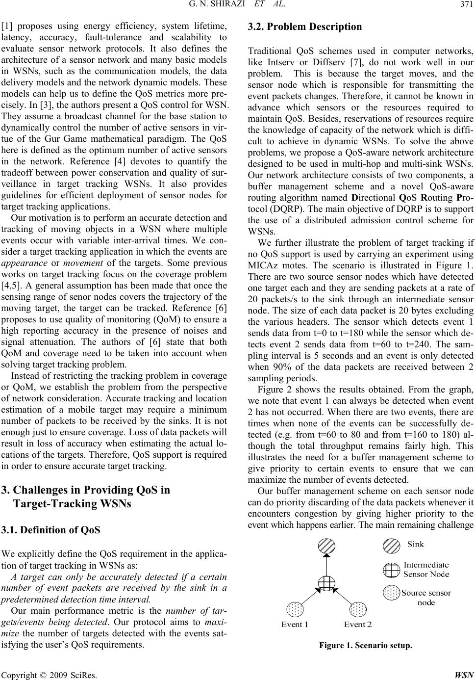

G. N. SHIRAZI ET AL.371
[1] proposes using energy efficiency, system lifetime,
latency, accuracy, fault-tolerance and scalability to
evaluate sensor network protocols. It also defines the
architecture of a sensor network and many basic models
in WSNs, such as the communication models, the data
delivery models and the network dynamic models. These
models can help us to define the QoS metrics more pre-
cisely. In [3], the authors present a QoS control for WSN.
They assume a broadcast channel for the base station to
dynamically control the number of active sensors in vir-
tue of the Gur Game mathematical paradigm. The QoS
here is defined as the optimum number of active sensors
in the network. Reference [4] devotes to quantify the
tradeoff between power conservation and quality of sur-
veillance in target tracking WSNs. It also provides
guidelines for efficient deployment of sensor nodes for
target tracking applications.
Our motivation is to perform an accurate detection and
tracking of moving objects in a WSN where multiple
events occur with variable inter-arrival times. We con-
sider a target tracking application in which the events are
appearance or movement of the targets. Some previous
works on target tracking focus on the coverage problem
[4,5]. A general assumption has been made that once the
sensing range of senor nodes covers the trajectory of the
moving target, the target can be tracked. Reference [6]
proposes to use quality of monitoring (QoM) to ensure a
high reporting accuracy in the presence of noises and
signal attenuation. The authors of [6] state that both
QoM and coverage need to be taken into account when
solving target tracking problem.
Instead of restricting the tracking problem in coverage
or QoM, we establish the problem from the perspective
of network consideration. Accurate tracking and location
estimation of a mobile target may require a minimum
number of packets to be received by the sinks. It is not
enough just to ensure coverage. Loss of data packets will
result in loss of accuracy when estimating the actual lo-
cations of the targets. Therefore, QoS support is required
in order to ensure accurate target tracking.
3. Challenges in Providing QoS in
Target-Tracking WSNs
3.1. Definition of QoS
We explicitly define the QoS requirement in the applica-
tion of target tracking in WSNs as:
A target can only be accurately detected if a certain
number of event packets are received by the sink in a
predetermined detection time interval.
Our main performance metric is the number of tar-
gets/events being detected. Our protocol aims to maxi-
mize the number of targets detected with the events sat-
isfying the user’s QoS requirements.
3.2. Problem Description
Traditional QoS schemes used in computer networks,
like Intserv or Diffserv [7], do not work well in our
problem. This is because the target moves, and the
sensor node which is responsible for transmitting the
event packets changes. Therefore, it cannot be known in
advance which sensors or the resources required to
maintain QoS. Besides, reservations of resources require
the knowledge of capacity of the network which is diffi-
cult to achieve in dynamic WSNs. To solve the above
problems, we propose a QoS-aware network architecture
designed to be used in multi-hop and multi-sink WSNs.
Our network architecture consists of two components, a
buffer management scheme and a novel QoS-aware
routing algorithm named Directional QoS Routing Pro-
tocol (DQRP). The main objective of DQRP is to support
the use of a distributed admission control scheme for
WSNs.
We further illustrate the problem of target tracking if
no QoS support is used by carrying an experiment using
MICAz motes. The scenario is illustrated in Figure 1.
There are two source sensor nodes which have detected
one target each and they are sending packets at a rate of
20 packets/s to the sink through an intermediate sensor
node. The size of each data packet is 20 bytes excluding
the various headers. The sensor which detects event 1
sends data from t=0 to t=180 while the sensor which de-
tects event 2 sends data from t=60 to t=240. The sam-
pling interval is 5 seconds and an event is only detected
when 90% of the data packets are received between 2
sampling periods.
Figure 2 shows the results obtained. From the graph,
we note that event 1 can always be detected when event
2 has not occurred. When there are two events, there are
times when none of the events can be successfully de-
tected (e.g. from t=60 to 80 and from t=160 to 180) al-
though the total throughput remains fairly high. This
illustrates the need for a buffer management scheme to
give priority to certain events to ensure that we can
maximize the number of events detected.
Our buffer management scheme on each sensor node
can do priority discarding of the data packets whenever it
encounters congestion by giving higher priority to the
event which happens earlier. The main remaining challenge
Figure 1. Scenario setup.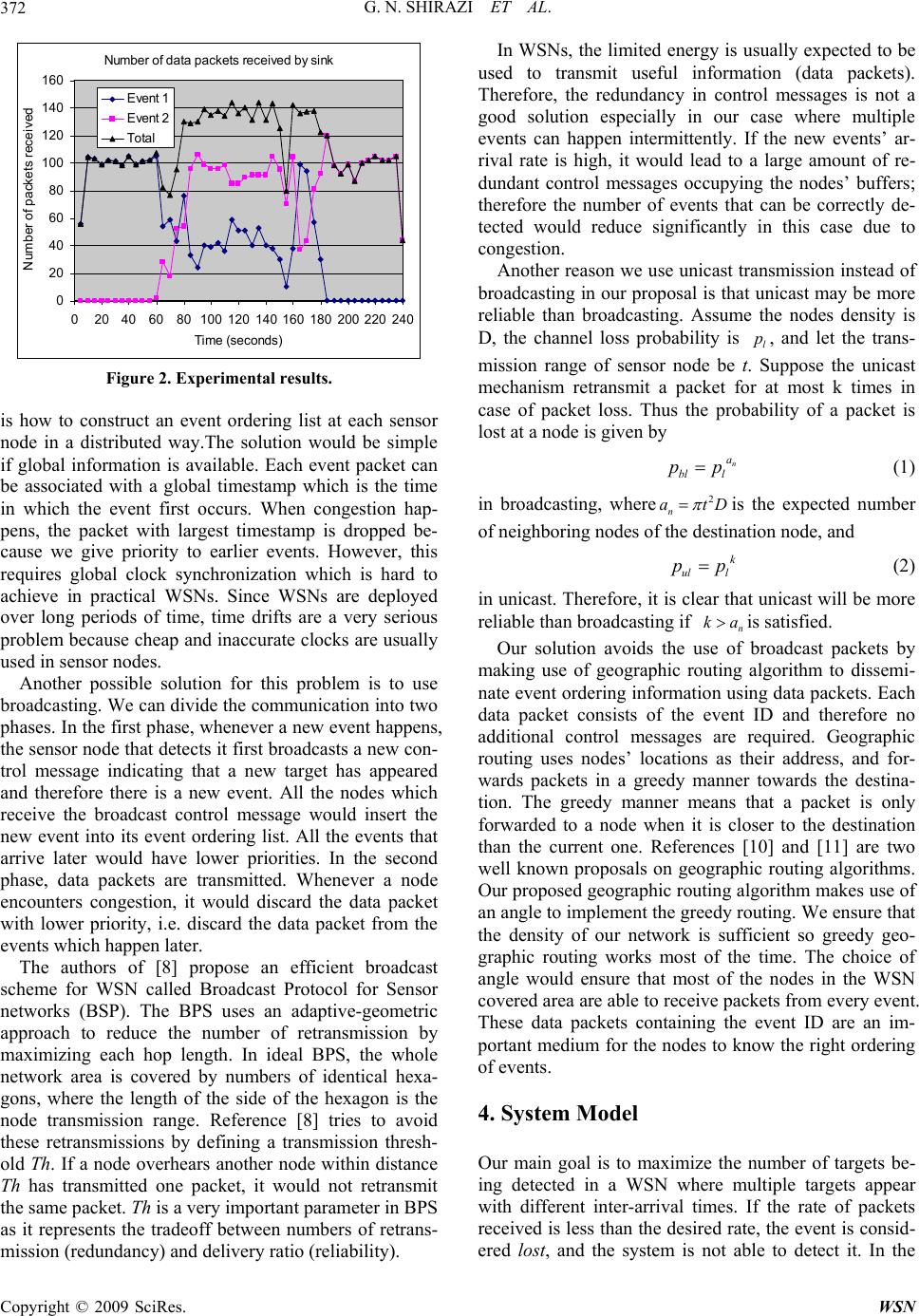

G. N. SHIRAZI ET AL. 372
Num ber of dat a packet s received by sin k
0
20
40
60
80
100
120
140
160
020406080100 120 140160 180 200220 240
T ime (seconds)
Number of packet s r eceived
Eve nt 1
Eve nt 2
Total
Figure 2. Experimental results.
is how to construct an event ordering list at each sensor
node in a distributed way.The solution would be simple
if global information is available. Each event packet can
be associated with a global timestamp which is the time
in which the event first occurs. When congestion hap-
pens, the packet with largest timestamp is dropped be-
cause we give priority to earlier events. However, this
requires global clock synchronization which is hard to
achieve in practical WSNs. Since WSNs are deployed
over long periods of time, time drifts are a very serious
problem because cheap and inaccurate clocks are usually
used in sensor nodes.
Another possible solution for this problem is to use
broadcasting. We can divide the communication into two
phases. In the first phase, whenever a new event happens,
the sensor node that detects it first broadcasts a new con-
trol message indicating that a new target has appeared
and therefore there is a new event. All the nodes which
receive the broadcast control message would insert the
new event into its event ordering list. All the events that
arrive later would have lower priorities. In the second
phase, data packets are transmitted. Whenever a node
encounters congestion, it would discard the data packet
with lower priority, i.e. discard the data packet from the
events which happen later.
The authors of [8] propose an efficient broadcast
scheme for WSN called Broadcast Protocol for Sensor
networks (BSP). The BPS uses an adaptive-geometric
approach to reduce the number of retransmission by
maximizing each hop length. In ideal BPS, the whole
network area is covered by numbers of identical hexa-
gons, where the length of the side of the hexagon is the
node transmission range. Reference [8] tries to avoid
these retransmissions by defining a transmission thresh-
old Th. If a node overhears another node within distance
Th has transmitted one packet, it would not retransmit
the same packet. Th is a very important parameter in BPS
as it represents the tradeoff between numbers of retrans-
mission (redundancy) and delivery ratio (reliability).
In WSNs, the limited energy is usually expected to be
used to transmit useful information (data packets).
Therefore, the redundancy in control messages is not a
good solution especially in our case where multiple
events can happen intermittently. If the new events’ ar-
rival rate is high, it would lead to a large amount of re-
dundant control messages occupying the nodes’ buffers;
therefore the number of events that can be correctly de-
tected would reduce significantly in this case due to
congestion.
Another reason we use unicast transmission instead of
broadcasting in our proposal is that unicast may be more
reliable than broadcasting. Assume the nodes density is
D, the channel loss probability is l
p, and let the trans-
mission range of sensor node be t. Suppose the unicast
mechanism retransmit a packet for at most k times in
case of packet loss. Thus the probability of a packet is
lost at a node is given by
n
a
bl l
pp (1)
in broadcasting, where2
n
at  D
is the expected number
of neighboring nodes of the destination node, and
k
ul l
pp (2)
in unicast. Therefore, it is clear that unicast will be more
reliable than broadcasting if n kais satisfied.
Our solution avoids the use of broadcast packets by
making use of geographic routing algorithm to dissemi-
nate event ordering information using data packets. Each
data packet consists of the event ID and therefore no
additional control messages are required. Geographic
routing uses nodes’ locations as their address, and for-
wards packets in a greedy manner towards the destina-
tion. The greedy manner means that a packet is only
forwarded to a node when it is closer to the destination
than the current one. References [10] and [11] are two
well known proposals on geographic routing algorithms.
Our proposed geographic routing algorithm makes use of
an angle to implement the greedy routing. We ensure that
the density of our network is sufficient so greedy geo-
graphic routing works most of the time. The choice of
angle would ensure that most of the nodes in the WSN
covered area are able to receive packets from every event.
These data packets containing the event ID are an im-
portant medium for the nodes to know the right ordering
of events.
4. System Model
Our main goal is to maximize the number of targets be-
ing detected in a WSN where multiple targets appear
with different inter-arrival times. If the rate of packets
received is less than the desired rate, the event is consid-
ered lost, and the system is not able to detect it. In the

G. N. SHIRAZI ET AL.373
following subsections, we describe different aspects of
our model, namely application, medium access control
(MAC), and physical (PHY) levels, as well as transport,
routing, and scheduling protocols. A distributed admis-
sion control scheme is then proposed in Section 5.
Each target is uniquely identified by a target ID, i. The
ith target, Ti, causes packet generation at a rate of ri in the
sensor nodes which detect it. Each event requires a
packet delivery requirement of i d. Therefore a mini-
mum packet rate of i dri is required at the sink for detec-
tion of the event.
The choice of MAC protocols and physical layer
characteristics (PHY) affect the capacity of the network,
C. However, it does not affect our goal of maximizing
the number of detected events given that the network
capacity is C. A higher C would lead to more events de-
tected and vice versa. Therefore, our QoS network archi-
tecture does not assume the use of any particular MAC
or PHY.
Our novel routing algorithm, DQRP, ensures that each
packet takes a different route to the sink such that after
β packets have been sent by the source, all the sensors
in the network will learn of the new event. Angle geo-
graphic routing is used and each data packet is given an
angle of routing
x
degrees. DQRP is further explained
in Section 5.
Each node maintains b buffers. Congestion occurs
when the number of packet arrivals exceeds the number
of buffers available, therefore buffer overflow occurs.
Each node maintains an event ordering list. Earlier
events are given higher priority when deciding which
packet to drop in the event of buffer overflow.
We consider a multiple sink architecture in which
sinks are able to share their received data. Therefore,
sensor nodes can choose any of the sinks as the destina-
tion. Moreover, we assume that the location of sinks and
neighboring sensors (i.e. sensor nodes within the trans-
mission range) are known. The arrival of events models a
Poisson Arrival Process. The targets stay in the WSN for
a period which follows an exponential distribution. Only
one sensor sends data packets to a sink for an event at
any given time.
5. Proposed QoS-Aw are Network Architecture
The main objectives and desired properties of our pro-
posed protocol are given as follows:
1) Path diversity: failure of a sink or failure of any
sensor node degrades performance gracefully. Any mali-
cious or selfish sensor node can only degrade perform-
ance gracefully.
2) Maintaining QoS: in event of congestion, earlier
events will get higher priority. This means that if event i
occurs before event j, if event i does not achieve the re-
quired QoS, event j also does not achieve the required
QoS.
3) Event Priority: In the event of congestion, event i
will take priority over event j if event i occurs before
event j.
A formal definition of an event being detected is given
as: An event is detected at time t if ii dr packets are re-
ceived in the interval [t-tmin, t] where tmin is the sampling
interval, di is the delivery ratio required by the user and
ri is the sending rate of the event.
This means that an event i is only detected at time t if
the sinks receive a minimum number of packets defined
by the QoS requirements of the user. The main perform-
ance metric is the number of events detected at a sam-
pling time and our goal is to maximize the number of
events detected. In addition, delay, throughput (total
amount of traffic received by the sinks), and energy
consumption should be considered as auxiliary perform-
ance metrics. Note that high throughput does not imply
that the number of events detected is high, as illustrated
in Figure 2.
5.1. Priority Buffer Management
We need to implement a priority buffer management
scheme in every node to ensure that if congestion occurs
and if we have the global event ordering list, we can de-
cide to give priority to certain events. Our priority buffer
management scheme is very efficient as insertion and
removal takes O(1) time.
5.2. DQRP Protocol
In this paper, we propose using a novel directional QoS
routing protocol (DQRP) to disseminate event ordering
information. In DQRP, the detection of an event is re-
ported to the entire network in order to provide QoS
management in case of congestion. More specifically,
when a target is first detected, the corresponding sensor
sends different data packets via different routes to the
multiple sinks. These routes are determined in such a
way that all nodes are informed about the existence of
the event after a certain time. The rationale behind in-
forming the entire network is to provide the network with
correct global event ordering, and hence enabling dis-
tributed admission control in the network.
To ensure that the maximum number of nodes can be
informed in an efficient way, it is required to find routes
to the sinks with the following two properties:
P1. Each node should be at least in one route.
P2. Number of shared nodes between every two routes
should be minimized.
In other words, a new data packet should inform a new
node about the event. Figure 3 shows two different set of

G. N. SHIRAZI ET AL. 374
routes. The left diagram on Figure 3 shows that some of
the intermediate nodes are not included in any route. In
contrast, the right diagram in Figure 3 shows all nodes
are included in at least one route.
In general, for a network topology where there are 4
sinks located at the edges of the network as shown in
Figure 3, we can divide the whole area into four quad-
rants. The key challenge is to determine the number of
packets to send to each sink and the paths of those data
packets should cover most of the nodes in the rectangle
region. Figure 4 shows a general situation of the four
quadrants in a 2 dimensional space. Assume the source
node locates at the origin (0,0), the destination sink lo-
cates at (x,y). Let the transmission range be t, and x=m't,
y=mt. First, we have the following lemma,
Lemma 1 The largest area of i
A, depending on m',
occurs at
''1
' or ('1)
mm
rmtr m

t (3)
where Ai=I(C(Rj))-I (C(Rj-1)). C(Ri) is the circle with
radius i
R
itand I(C) is defined as the intersected region
of C with the rectangle. The value corresponding
to i (A )Max is (whichever is larger):
*2
*21 21
'1'1 ''
22 22
'1 '
A(21)/4
A[sin(/)sin(/)
]/2
mmm
mm
tm
orrxrrx r
xrx xrx







m
(4)
Figure 3. Two different set of routes from the source node
to the sinks.
Figure 4. Intersection between transmission range spheres
and the rectangle between the source (u) and the sink (s).
Proof: Denote area by | |. If Ri ≤ mt, the area of i A is
given by
1
2
A(|| ||)/4
=t(21)/ 4
iii
CR CR
i 


 (5)
If Ri > mt, then the area is computed by dividing it to
an arc and a right triangle, and is given by
11
A(|( )||()|)(|()| |()|)
iii ii
Arc RTRArc RTR

 
(6)
where T(Ri) is the right triangle with hypotenuse equal to
Ri and Arc(Ri) is I(C(Ri))- T(Ri). It is easy to find
|()
i|
A
rc R and |( |, and they are given by )
i
TR
21
'
22
|()| sin(/
|()|]/2
im i
ii
)
A
rc Rrxr
TRxrx



(7)
Substituting (5) in (4) gives
21 21
11
22 22
1
A[sin(/)sin(/)
]/2
iii ii
ii
rxrrx
xrx xr x





r
(8)
By taking derivatives of (5) and (8), it turns out that (5)
is a increasing function of Ri, while (8) is a decreasing
function of Ri. Thus, the maximum occurs either
when ''
im
rr mt

 (max. of (5)) or when''
im
rr mt


(max. of (8)).
Next, we present our general angle dividing algorithm.
The proposed angle dividing algorithm guarantees that in
each routing area that divided by angle12 ,,..., l

 , the
largest number of nodes that need to receive distinguish-
ing data packets are close to and bounded by
upp upp
aSD

(9)
where upp a denotes upper bound of the number of nodes,
upp
S denotes the upper bound of area of the region, and
D is the nodes density of the WSN. We use A to denote
region, S to denote area and assume the transmission
range is t. The algorithm is presented in Algorithm 1. We
explain Algorithm 1 by a simple example in Figures 5,6.
The main idea is that the angles should be chosen such
that the shadowed regions share the same area upp S. It
should be noted that the value of upp
S will affect the
delivery ratio as well as the convergence speed of our
angle routing algorithm. A larger value of upp
S allows
larger angles 12 ,,..., l

 to exist. A larger angle may
increase the delivery ratio in the sense that if a data
packet for a node in the shaded area is lost, other pack-
ets that share the same path before reaching the shaded
area can serve as the informers. For example, in Figure
6, node 4 and node 5 will share the same intermediate
node, node 0 and node 1. If a packet being sent to
node 5 is lost at node 0, node 0 and node 1 can still learn
θi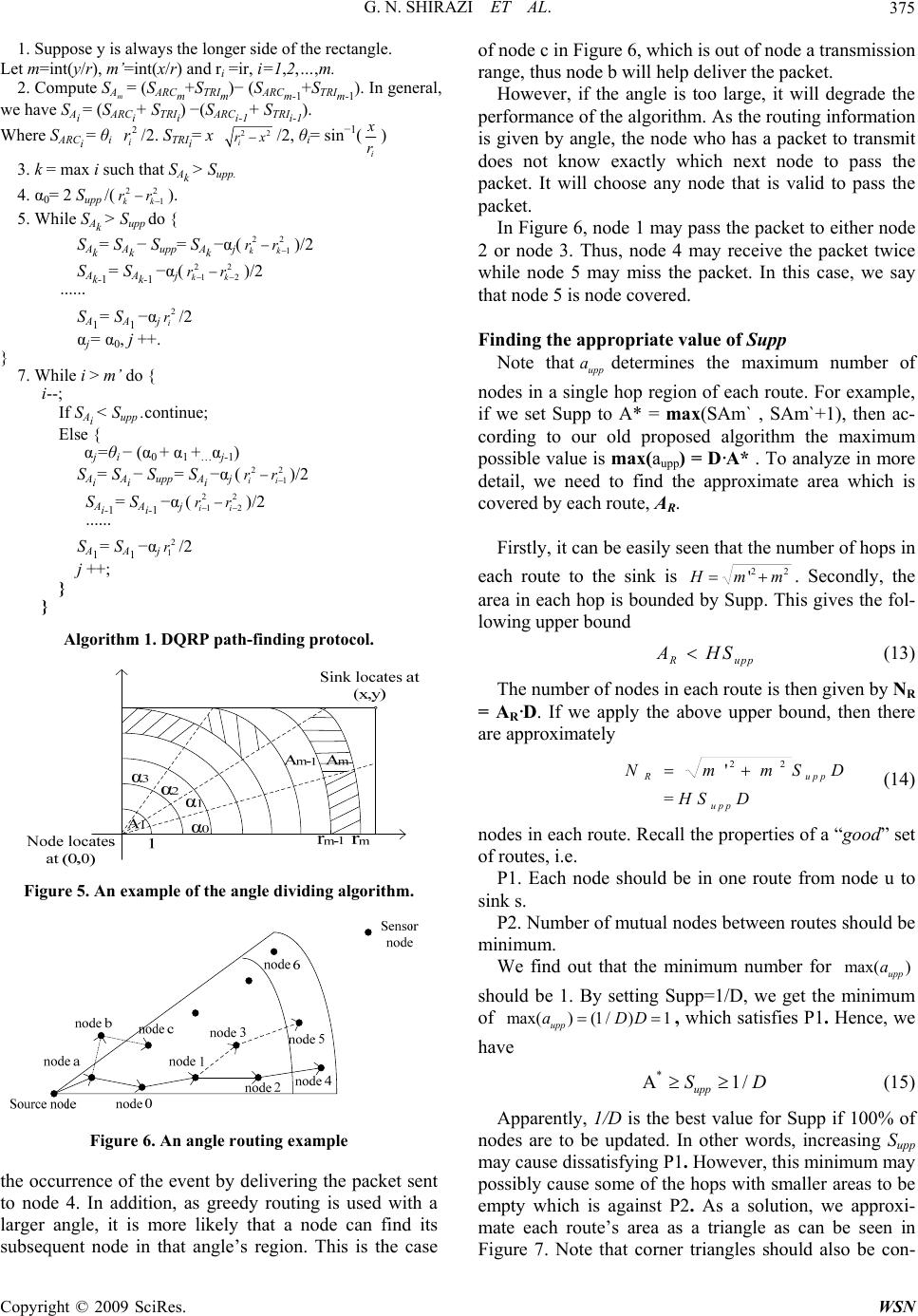

G. N. SHIRAZI ET AL.375
1. Suppose y is always the longer side of the rectangle.
Let m=int(y/r), m’=int(x/r) and ri =ir, i=1,2,…,m.
2. Compute SAm = (SARCm+STRIm)− (SARCm-1+STRIm-1). In general,
we have SAi = (SARCi+ STRIi) −(SARCi-1+ STRIi-1).
Where SARCi = θi /2. STRIi= x
2
i
r22
i
rx/2, θi= sin−1(
i
x
r)
3. k = max i such that SAk > Supp.
4. α0= 2 Supp /().
22
1kk
rr


5. While SAk > Supp do {
SAk= SAk − Supp= SAk −αj()/2
22
1kk
rr


2
SAk-1= SAk-1 −αj()/2
2
1kk
rr

2
2
······
SA1= SA1 −αj/2
2
i
r
αj= α0, j ++.
}
7. While i > m’ do {
i--;
If SAi < Supp .continue;
Else {
αj=θi − (α0 + α1 +…αj-1)
SAi= SAi − Supp= SAi −αj ()/2
22
1ii
rr


2
SAi-1= SAi-1 −αj ()/2
2
1ii
rr


······
SA1= SA1 −αj/2
2
1
r
j ++;
}
}
Algorithm 1. DQRP path-finding protocol.
Figure 5. An example of the angle dividing algorithm.
Figure 6. An angle routing exam ple
the occurrence of the event by delivering the packet sent
to node 4. In addition, as greedy routing is used with a
larger angle, it is more likely that a node can find its
subsequent node in that angle’s region. This is the case
of node c in Figure 6, which is out of node a transmission
range, thus node b will help deliver the packet.
However, if the angle is too large, it will degrade the
performance of the algorithm. As the routing information
is given by angle, the node who has a packet to transmit
does not know exactly which next node to pass the
packet. It will choose any node that is valid to pass the
packet.
In Figure 6, node 1 may pass the packet to either node
2 or node 3. Thus, node 4 may receive the packet twice
while node 5 may miss the packet. In this case, we say
that node 5 is node covered.
Finding the appropriate value of Supp
Note thatupp adetermines the maximum number of
nodes in a single hop region of each route. For example,
if we set Supp to A* = max(SAm` , SAm`+1), then ac-
cording to our old proposed algorithm the maximum
possible value is max(aupp) = D·A* . To analyze in more
detail, we need to find the approximate area which is
covered by each route, AR.
Firstly, it can be easily seen that the number of hops in
each route to the sink is 22
'Hmm
. Secondly, the
area in each hop is bounded by Supp. This gives the fol-
lowing upper bound
R
upp
A
HS

(13)
The number of nodes in each route is then given by NR
= AR·D. If we apply the above upper bound, then there
are approximately
22
'
=
R upp
upp
NmmS
HS D
 D
(14)
nodes in each route. Recall the properties of a “good” set
of routes, i.e.
P1. Each node should be in one route from node u to
sink s.
P2. Number of mutual nodes between routes should be
minimum.
We find out that the minimum number for max( )
upp
a
should be 1. By setting Supp=1/D, we get the minimum
of max()(1/)1
upp
aDD

, which satisfies P1. Hence, we
have
*
A1
upp
S/D (15)
Apparently, 1/D is the best value for Supp if 100% of
nodes are to be updated. In other words, increasing Supp
may cause dissatisfying P1. However, this minimum may
possibly cause some of the hops with smaller areas to be
empty which is against P2. As a solution, we approxi-
mate each route’s area as a triangle as can be seen in
Figure 7. Note that corner triangles should also be con-

G. N. SHIRAZI ET AL. 376
tinued to the sink, so we assume that each of these trian-
gles has a height equal to /
upp
St, and a base equal toHt .
Thus we have
/2
= /2
R upp
upp
A
HtS t
HS
 (16)
To satisfy P1 and P2, it is required to set R
NH

.
Therefore we have /2
R Rupp
NADHSD , which implies
2/
upp
SD (17)
It should be also noted that for larger values of upp
S,
P1 might not be satisfied due to the fact that the number
of nodes may be increased to more than one and hence,
be omitted from the routes. However, for larger values of
upp
S, it is more unlikely to have same node receives the
packet twice (i.e. satisfying P2).
Another important point is that if we assume we have
only local information, then density D may not known at
each node. We can either assume that we have D (non
local info), or estimate it using
2
est
D=N / (/4)
uu
neib t
 (18)
where Nu
neib denotes the number of neighbors of node u.
6. Delay Analysis
6.1. Propagation Delay
The propagation delay, the approximate delay is propor-
tional to22 'Hmm. Therefore, transmission delay is
proportional to distance between source and the sink, dt
= c H, where c is the average propagation delay for one
hop transmission.
6.2. Priority Queue delay
When there is buffer management in nodes, the packet
sees an average delay, ds, at each hop. ds depends on
Figure 7. Approximating the r outes with triangles.
A
ver age Event Thr oughput Wit ho ut ( 1) and W i t h (2)
Buff er Manageme nt
0
0.1
0.2
0.3
0.4
0.5
0.6
0.7
0.8
0.9
1
12
Case
Throughput
Event 1
Event 2
Figure 8. Normalized throughput of 2 events with simple
queue management (case 1) and priority queue (case 2).
congestion level and also the priority of the packet. In
[12], an analysis for the average delay in a non- preemp-
tive Head of Line (HOL) priority queue is given. A
non-preemptive HOL queue has the property that the
packet in the head of line, which is being processed by
the server, should be completely served before other
packets can be processed. Using the results (Equation (9)
in [12]) and simplifying it for a HOL M/M/1 priority
queue, we get the following formula. 1
11
111
1
11
12(1)(1
iii
mm
mmn
ii Mii
mm
mmm
ds


1
)
n
m







 



(19)
where i

is the average service time for i’th priority
class; M is the total number of priority classes; and i

is the offered load of packets in priority class i. Denoting
the packet arrival rate of priority class i by i

,i

is
defined as iii



. In general, a smaller index for a
priority class implies a higher priority, and hence less
delay for that class. In fact, from the Equation (10), it can
be seen that the first class packets observe the least delay
( i.e.1 ds 1


). More importantly, this delay is less than
the delay in a queue without prioritizing (1 '1 ds


).
The fact that ds1 < ds', shows that the more important
packets leave the queue quickly. On the other extreme
hand, the delay for last priority class dsM is obviously
larger than ds', and hence, the packets from less impor-
tant class observe more delay compared to non- priori-
tized mode.
1The second and third terms in the right hand side of the Equation (1)
should also have the same unit as i

by multiplying them into 1 time
unit.

G. N. SHIRAZI ET AL.377
dsi is the queuing delay for one hop only. Similar to
what we had for the propagation delay, the total queuing
delay will be dqi = H dsi.
Figure 8 shows the effect of implementing a simple
priority queue scheme on the throughput from two dif-
ferent priority classes. The setting is similar to Figure 2
when both events are active. As can be seen, after apply-
ing the buffer management, the class 1 packet will have
more throughput compared to normal queue management.
For example, if 0.9
i

, then the first event can be de-
tected with the priority queue management in contrast to
normal queue management.
6.3. Total Delay
The total delay is given by di = dt + dqi = H (c + dsi).
Therefore, for the packets in a certain priority class, the
nearest sink to the node observes the least delay. Hence,
after disseminating of the information about the exis-
tence of one event by the proposed angle routing, the
nearest sink can be used in order to achieve the least
possible delay. The data dissemination phase guarantees
that the maximum number of events is detected, because
of the global event ordering knowledge in the network.
7. Analysis of Our Protocol
At first glance, our DQRP protocol seems to reduce the
throughput or the number of events detected because the
average number of hops per event packet increases. We
should prove using linear programming to show that
DQRP can actually increase our performance metric
which is the number of targets detected. Shortest-path
greedy geographic routing is not optimal in multi-sink
sensor networks.
We consider a n×n grid topology of sensor nodes with
4 sinks located at the corners of the grid. The sensor
network can be modeled using the representation of a
graph G=(V,E) where V is the set of vertices and E is the
set of edges. The sink and all sensor nodes are in the set
of vertices. Each vertex is associated with a location in-
formation given by (xi, yi). Each sensor node has a
maximum transmission range of t There is an edge (u, v)
in E if the nodes are within transmission range of each
other. Formally, this is stated as
Edge 22
, ()()
uv uv
uv Eiffxxyyt
Data is sent from a sensor node through intermediate
sensor nodes to the sink if the sink is not within direct
transmission range of the sensor. We let(,)
f
uv be the
total amount of data transmitted from sensor node u to
sensor node v. These data includes data from other sen-
sor nodes and data originating from the node itself. We
let G be a weighted graph with a weight function w. The
weight (,)
f
uvD, (, )wuv of the edge ,uvED is the cost
of transmission from node u to node v. The transmission
cost is dependant on the distance between the nodes as
well as the propagation model used. In general,
(,) k wuv d

where d is the distance between 2 nodes and k
is the path loss exponent. We let k be 2 in our scenario.
As we consider only a static grid topology, w(u,v) is a
fixed value. We consider 3 types of routing:
1) Nearest-sink Greedy Geographic Routing: This
means that the node will choose the nearest sink to send
the data packets to and the next hop it chooses will
maximize the distance gained towards the sink.
2) Nearest-sink Non-Greedy Geographic Routing:
This means that the node will choose the nearest sink to
send the data packets to and it can choose any neighbor
which is nearer to the sink than it is to forward the data
packets.
3) Multi-sink Non-Greedy Geographic Routing: This
means that the node can choose any sink to send the data
packets to and it can choose any neighbor which is
nearer to the target sink than it is to forward the data
packets. We minimize the maximum energy consumed
by any sensor node by linear programming:
7.1. Nearest-Sink Greedy Geographic Routing
Minimize p subject to the following constraints:
0
f
(u,v) = for each (u,v) E (20)
0Df(u,v)  for each (u,v) E and v maximizes dis-
tance gained towards the nearest sink of u (21)
vV
f
(u,v) c



for each u- {sink} (22) V
u
vV vV
f
(u,v)f(v,u)= L



 for each uV- {sink} (23)
0
vV
f
(u,v)=


for u{sink} (24)

sink sink
u
uvV uV
f
(v,u)= L
 


u{sink} (25)
vV
f
(u,v)w(u,v) p



uV- {sink} (26)
The variable c is the maximum amount of data trans-
mitted by any sensor node among all the sensor nodes in
the network. Constraint (20) means that if two sensor
nodes are not within the transmission range, the flow
between each other is 0. If two sensor nodes are within
transmission range, the flow between each other must be
non negative as stated in Constraint (21). Constraint (21)
will vary based on the type of routing algorithm used.
Constraint (22) states that the total amount of transmis-
sion data by any sensor node cannot exceed c. We set c
to be 10 packets of data. Constraint (23) states that all
received data are to be forwarded and every sensor node
has u
Lunits of data to be sent to the sink. This value

G. N. SHIRAZI ET AL. 378
depends on the number of event packets assigned to that
node. Constraints (24) and (25) states that the sink is not
sending any data and should receive all the data from the
sensor nodes. Constraint (26) states that if the linear pro-
gramming problem can be solved, the solver should
produce a solution that minimizes the energy consump-
tion of the sensor nodes.
7.2. Nearest-Sin k Non-Greedy Ge ographic Routing
The linear program is similar to the previous case but (28)
is modified.
Minimize p subject to the following constraints:
0
f
(u,v)= for each (u,v) E (27)
0
f
(u,v) for each (u,v) E

and v is nearer to the
nearest sink than u is (28)
vV
f
(u,v) c


 for each u- {sink} (29)
V
u
vV vV
f
(u,v)f(v,u)= L


 for each uV- {sink}(30)
0
vV
f
(u,v)=

 for u{sink} (31)

sink sink
u
uvV uV
f
(v,u)= L
 
 for u{sink} (32)
vV
f
(u,v)w(u,v) pd


for each uV- {sink} (33)
7.3. Multi-sink Non-Greedy Geographic Routing
The linear program is similar to the previous case but (35)
is modified.
Minimize p subject to the following constraints:
0
f
(u,v)= for each (u,v) E (34)
0 f(u,v)  for each (u,v) E (35)
vV
f
(u,v) c


 for each u- {sink} (36)
V
u
vV vV
f
(u,v)f(v,u)= L


 uV-{sink} (37)
0
vV
f
(u,v)=

 for u{sink} (38)

sink sink
u
uvV uV
f
(v,u)= L
 
 , u {sink} (39)
vV
f
(u,v)w(u,v) p


for each uV- {sink} (40)
We vary the number of packets generated by each
event and determine the maximum number of events
which can satisfy the QoS. Each event is randomly as-
signed to sensor nodes. The transmission range is set to
5 by 5 G rid Topology
0
20
40
60
80
100
120
140
12345678910
P ac ket rate of eac h event (packets/s)
M ax im um num ber of ev ent s
Nearest Sink , G reedy G eographic
Routi ng
Nearest Sink , Non-Greedy
Geographic Rout i ng
Mul ti -S i nk, Non-Greedy Geographi c
Routi ng
Figure 9. Maximum number of events satisfying QoS re-
quirements in a 5 by 5 grid topology.
6 by 6 G ri d
0
20
40
60
80
100
120
140
12345678 910
P acket s endi ng rate of eac h event (packet / s)
M ax im um num ber of ev ent s
Neares t Si n k , Greedy Geographi c
Rout i ng
Neares t Si n k, Non-Greedy
Geographi c Rout i ng
M ul t i -S i nk, Non-Greedy
Geographi c Rout i ng
Figure 10. Maximum number of events satisfying QoS re-
quirements in a 6 by 6 grid topology.
2, therefore each node has 8 neighbors. The maximum
number of events is reached when the solver cannot find
a solution to the linear program. We use the solver in
MATLAB for this analysis. Figure 9 shows the maxi-
mum number of events satisfying the QoS requirements
for a 5 by 5 grid topology and Figure 10 shows the re-
sults for a 6 by 6 grid topology. These results show that
multipath non-greedy geographic routing can indeed
improve network performance.
8. Implementation Results
We test the effectiveness of our priority queue buffer by
implementing the scheme on the MICAz motes. In the
first scenario, we use 3 motes in which there is 1 sink
and 2 traffic sources as shown in Figure 11. In the second

G. N. SHIRAZI ET AL. 379
Figure 11. Network topology in scenario 1.
Throughput of eac h event without pri ority buffer
0
20
40
60
80
100
120
020406080100 120140 160180200220240
Tim e (s econds)
Number of packets receive
d
E vent 1
E vent 2
Figure 12. Throughput of events without priority buffer.
Throughput of each event wit h pri orit y management
0
20
40
60
80
100
120
020406080100120140 160180 200 220 240
Ti m e (seconds)
Num ber of pac k ets rec eiv ed
Event 1
Event 2
Figure 13. Throughput of events with priority buffer.
scenario, we use a total of 18 motes in which there is 1
sink and 5 traffic sources. The nodes are randomly de-
ployed in a lab. Each mote is between 1 to 5 hops away
from the sink. Each event sends packets at a rate of 20
packets per second for the first scenario and 10 packets
per second. The sampling interval is set to 5 seconds.
Figure 12 shows the number of packets received by
each event when there is no priority buffer management
scheme and Figure 13 shows the number of packets re-
ceived by each event when there is priority buffer man-
agement scheme. Figure 14 shows the number of events
detected based on our QoS requirements. It can be
clearly seen that the priority management scheme im-
proves QoS performance. In the random deployment
scenario, each event is gradually introduced into the
network until there are 5 events.
After that, events gradually leave the network. Figure
15 shows the number of events detected. The results
show that our priority buffer management scheme per-
forms better most of the time.
One of the main problems that we face when carrying
out the experiments is that the experiment was done in a
lab where shadowing and fading effects are more serious
compared to an open field. This causes the link quality to
vary rapidly. As a result, there are a lot of fluctuations in
the number of packets received and routes between
nodes change quite often. Our scheme could potentially
improve the performance much higher if the experiment
is carried out in an open environment (e.g. open field)
where there are less obstacles and the link quality is
more stable.
S cenario 1
0
1
020406080100120 140160 180 200220240
Tim e (sec onds)
Number of events detec ted
Wit hout Priority
Buffer
With Priority
Buffer
Figure 14. Number of events satisfying our QoS require-
ments. The required data delivery ratio is 90%.
Random Deploym ent Scenario
0
1
2
3
0306090120 150 180210 240 270 300 330360 390 420 450480 510 540
Tim e (s econds )
Num ber of events detec ted
Without Priority Buffer
With Priority Buffer
Figure 15. Number of detected events in a random deploy-
ment scenario satisfying our QoS requirements. The re-
quired data delivery ratio is 70%.

G. N. SHIRAZI ET AL. 380
Number of Det ec ted E vents(data deli very rat io=0.9)
0
1
020406080100 120 140160 180
time(s)
Number of events detecte
d
DQRP
Base
Number of Det ec ted Events(data deli very= 0.8)
0
1
2
020406080100120140 160 180
time(s)
Num ber of event s detec ted
DQRP
Base
(a) (b)
Number of Detec ted E vents(data deli very rat i o=0. 7)
0
1
2
020406080100 120 140160 180
time(s)
Numb er of E vents
DQRP
Base
Number of Detected Events(data delivery ratio=0.6)
0
1
2
020406080100 120 140 160 180
ti me (s )
Number of Events
DQRP
Bas e
(c) (d)
Figure 16. Number of detected events, out of max. 4 events, in the basic setup (stars) and DQRP (triangles). Vertical axis
shows the number of events detected, and horizontal axis shows the time. The required data delivery ratio for an event detec-
tion at sinks is a) 0.9, b) 0.8, c) 0.7, and d) 0.6.
9. Simulation Results
We simulate a network consisting of 25 nodes with
DQRP and using priority buffer management scheme
based on event ordering. The simulation tool used is
TOSSIM. There are 4 sinks located at each corner of the
simulation area. We simulate two scenarios, one with 4
events and another with 8 events. Events are gradually
inserted into the network. Events can also leave the net-
work after some time. The sampling interval is 2 seconds.
We compare the number of events detected with varying
QoS requirements from 60% delivery ratio to 90% de-
livery ratio. The results for the scenario with 4 events are
shown in Figure 16 and the results for the scenario with 8
events are shown in Figure 17. The results show that
DQRP with priority buffer management scheme based on
event ordering achieves better performance.
10. Conclusions and Future Work
In this paper, we have presented a QoS network archi-
tecture for target tracking WSNs consisting of a priority
buffer management scheme based on event ordering and
a routing algorithm to disseminate the event ordering.
We believe that better performance can be obtained
from our system by using cross-layer design. For exam-
ple, once we have the global event-ordering list, at the
MAC layer, we can assign more time slots using a
TDMA MAC protocol to events that have a higher prior-
ity. This can provide more assured QoS than the CSMA
MAC protocol that is used in our simulations and ex-
periments.

G. N. SHIRAZI ET AL.381
Numb er of Det ecte d Events(da ta d el ivery rati o=0.9)
0
1
2
3
020406080100 120 140160 180 200
time(s)
Number of E vents
DQRP
Base
Number of Detec ted E vents(data deli very rat i o=0. 8)
0
1
2
3
020406080100 120 140 160180 200
time(s)
Number of E vents
DQRP
Base
(a) (b)
Numbe r of Det ected Event s(data deli very rati o=0.7)
0
1
2
3
020406080100 120140 160180 200
time(s)
Number of Event
s
DQRP
Base
Number of Det ected E vent s(dat a deli very rat i o=0.6)
0
1
2
3
020406080100 120 140160 180 200
time(s)
Number of Ev ent s
DQRP
Base
(c) (d)
Figure 17. Number of detected events, out of max. 8 events, in the same format as Figure 16.
11. References
[1] S. Tilak, N. B. Abu-Ghazaleh, and W. Heinzelman, “A
taxonomy of sensor network communication models,”
ACM Mobile Computing & Communication Review, Vol.
6, No. 2, pp. 1−8, 2002.
[2] D. Chen and P. K. Varshney, “QoS support in wireless
sensor networks: A survey,” Proceedings of the 2004 In-
ternational Conference on Wireless Networks (ICWN
2004), Las Vegas, Nevada, USA, June 2004.
[3] R. Iyer and L. Kleinrock, “QoS control for sensor net-
works,” Proceedings of IEEE International Conference on
Communications (ICC’03), Vol. 1, pp. 517−521, May
2003.
[4] C. Gui and P. Mohapatra, “Power conservation and qual-
ity of surveillance in target tracking sensor networks,”
ACM International Conference on Mobile Computing
and Networking (MOBICOM), 2004.
[5] Q. X. Wang, W. P. Chen, R. Zheng, K. Lee, and L. Sha,
“Acoustic target tracking using tiny wireless sensor de-
vices,” In International Workshop on Information Proc-
essing in Sensor Networks (IPSN), 2003.
[6] G. H. He and J. C. Hou, “Tracking targets with quality in
wireless sensor networks,” proceedings of the 13th IEEE
International Conference on Network Protocols, 0-7695-
2437−8/05, 2005.
[7] K. I. Park, “QoS in packet networks,” Springer, pp. 159−
179, 2005.
[8] A. Durresi, V. K. Paruchuri, S. S. Iyengar, and R. Kannan,
“Broadcast protocol for sensor networks,” Technical Re-
port, LSU-CSC, October 2003.
[9] A. Durresi, V. K. Paruchuri, L. Barolli, and R. Jain,
“Qos-energy aware broadcast for sensor networks”, Pro-
ceeding of the 8th IEEE Int. Symp. on Parallel Architec-
tures, Algorithm and Networks (ISPAN’05), 1087−
4089/05, 2005.

G. N. SHIRAZI ET AL. 382
[10] P. Bose, P. Morin, I. Stojmenovic, and J. Urrutia, “Rout-
ing with guaranteed delivery in Ad-Hoc wireless net-
works,” ACM Wireless Networks, November 2001.
[11] B. Karp and H. T. Kung, “GPSR: Greedy perimeter state-
less routing for wireless networks,” ACM/IEEE Int. Conf.
on Mobile Computing and Networking (Mobicom), 2000.
[12] J. Walraevens, B. Steyaert, M. Moeneclaey, and H.
Bruneel, “Delay analysis of a HOL priority queue,”
Telecommunication Systems, Vol. 30, No. 1–3, pp. 81–
98, 2005.
[13] G. N. Shirazi, P. Wang, D. Xiangxu, Z. A. Eu, and C. K.
Tham, “A QoS network architecture for multi-hop
multi-sink target Ttracking WSNs,” IEEE Inte Conference
on Communication Systems (ICCS), pp. 17−21, 2008.