Journal of Water Resource and Protection
Vol.6 No.4(2014), Article ID:44276,8 pages DOI:10.4236/jwarp.2014.64034
Comparison of Different Ann Approaches in Daily Pan Evaporation Prediction
Yildirim Dalkiliç1, Umut Okkan2, Nesrin Baykan3*
1Department of CE, Faculty of Engneering, Erzincan University, Erzincan, Turkey
2Department of CE, Faculty of Engneering, Balikesir University, Balıkesir, Turkey
3Department of CE, Faculty of Engneering, Pamukkale University, Denizli, Turkey
Email: yildirim.dalkilic@gmail.com, uokkan@balikesir.edu.tr, *nesribaykan61@gmail.com
Copyright © 2014 by authors and Scientific Research Publishing Inc.
This work is licensed under the Creative Commons Attribution International License (CC BY).
http://creativecommons.org/licenses/by/4.0/


Received 22 January 2014; revised 21 February 2014; accepted 15 March 2014
ABSTRACT
Nowadays, one of the most important effects on water resources under climate change is increasing of free water surface evaporation which depends on the increasing of temperature. In basins, where there are no observed data, free water surface evaporation is taken into account depending on historical temperature and similar data and their long-term statistics. Predicting of real value of evaporation contains some uncertainties. The modeling of evaporation with a small number of predictors has crucial importance on the regions and basins where measurements are not sufficient and/or not exist. In this presented study, daily evaporation prediction models were prepared by using empirical Penman equation, Levenberg-Marquardt algorithm based on "Feed Forward Back Propagation Artificial Neural Networks (LMANN)", radial basis neural networks (RBNN), generalized regression neural networks (GRNN). When the models were compared, it was noticed that the results of neural network models are statistically more meaningful than the Penman equation.
Keywords:Daily Evaporation; Pan Evaporation; Evaporation Prediction; Penman; LMANN; RBNN; GRNN

1. Introduction
Climate change becomes more and more important and effects hydrologic circle and water resources day by day. Evaporation is one of the most important parameters of hydrologic circle and its prediction is getting more important because of climate change effects. Both designing the water works and planning and management of water resources systems, modeling of evaporation have significant importance. The modeling of evaporation, being one of its most prominent predictor, is of crucial importance on the regions and basins where measurements are not sufficient or are not exist.
The purpose of this study is to apply different ANN techniques and compare them with Penman-Monteith method in order to estimate daily pan evaporation and reference evapotranspiration. FAO suggests PenmanMonteith Method to estimate daily evaporation as standard and this method is widely used in the world but it requires many parameters. We investigated that if modeling of daily pan evaporation with using much less parameters than Penman-Monteith, is possible and compared the results of employed ANN techniques including Levenberg-Marquardt algorithm based Feed Forward Back Propagation neural networks (LMANN), radial basis neural networks (RBNN), generalized regression neural networks (GRNN).
There are many studies about modeling of evaporation and reference evapotranspiration. Reference [1] investigated the utility of ANN for estimation of daily grass reference crop evapotranspiration (ETo) and compared the performance of ANNs with the conventional method (Penman-Monteith) used to estimate ETo. Reference [2] attempted to find best alternative method to estimate reference evapotranspiration by using Penman-Monteith and ANN techniques. Reference [3] developed and applied generalized regression neural network model embedding the genetic algoratihm in order to estimate and calculate the pan evaporation (PE) and reference (ETr) evapotranspiration. Reference [4] applied ANN first time to estimate evaporation in hot and dry region (BWh climate by the Köppen classification). Reference [5] applied the radial basis function (RBF) network for pan evaporation to evapotranspiration conversions. Reference [6] modeled variation in solar radiation, vapor pressure deficit and soil moisture by using Jarvis-Stewart model and then they also modeled canopy conductance and estimated transpiration via the PM model. It is also important study of modeling of evaporation and evapotranspiration.
Reference [7] estimated daily pan evaporation by using ANN techniques and they estimated daily pan evaporation by using classical approach such as Priestley-Taylor, Brutsaert-Stricker, Makkink and Hamon methods and compared the results. Reference [8] assessed the ability of three models of Local Linear Regression (LLR), Support Vector Machine (SVM) and Artificial Neural Network (ANN) to estimate evaporation from reservoirs as one of the critical components of hydrological cycle in arid and semi-arid regions. Reference [9] proposed a self-organizing map neural network (SOMN) to assess the variability of daily evaporation based on meteorological variables.
2. Applied Methods
Evaporation, which changes related with energy, mass and energy transfer mechanism, water depth and surface area, is basic component of hydrological circle and the function of radiation, temperature, wind speed, relative humidity and atmospheric pressure [10] . Evaporation can directly measured by evaporimeter or can predicted by empirical equations such as in [11] .
In this study, the availability of ANN models, which is developed as an alternative technique against to empirical methods such as Penman, were examined. Penman needs complex calculations and too many parameters belongs to study area, but ANN can obtain more significant results with less parameters than empirical equations such as Penman. ANN is an artificial technique which developed by using properties of neural system such as definition, prediction and reproduce of knowledge [12] . It is possible to come across too many algorithm types which developed within ANN. In this study, three different ANN algorithm; Levenberg-Marquardt algorithm which is one of the feed forward back propagation algorithm [13] , Radial Basis Neural Network (RBNN) [14] and Generalized Regression Neural Network (GRNN) [15] were used. Details of method were presented by Okkan and Dalkılıç [16] [17] .
3. Application and Findings
Daily mean temperature (Tmean) and relative humidity (RHmean), wind speed at 2 m level (Wmean), maximum and minimum temperatures (Tmax, and Tmin) and total solar radiation (Rad) have been used as input-data for Penman-Monteith equation and ANN-models have been set by using these inputs. In order to examine the generalization-abilities of ANN-models, the models have been set by using 70% of data for training and tested by remaining data-set. At this stage, MATLAB codes have been used written by the authors. In order to increase the performance of the models and the speed of their convergence during the training period, all data have been scaled at the range of 0 - 1 and given to the networks. The scaled data have been converted to their original values by inverse operation after the completion of training process. By the training of the models, parameters related to algorithms and network structures have been determined so that the mean square errors (MSE) have to converge to a minimum while coefficient of determination (R2) to a maximum.
By the training of Levenberg-Marquardt ANN (LMANN), Levenberg-Marquardt Standard Error (LMSE) value has been obtained by using cell number of hidden layer is 5, the first value of Marquardt parameter (μ0) is 0.001 and decay rate (β) is 0.1. Furthermore, ten iterations have been found satisfactorily because of to prevent deterioration of test period performances as a result of extreme learning of LMANN model. Sigmoid function was selected as activation function in LMANN model (Equation (1)) by the training of,
 (1)
(1)
The results of LMANN model were evaluated by using scatter diagrams and in terms of statistical parameters. Scatter diagrams of testing and training periods of LMANN model are presented in Figure 1.
In training period of RTANN, cell number in hidden layer is selected as 5 and σ is determined so as to find minimum mean square error. Accordingly, optimum σ value is found as 0.85. In this model, Gauss function is selected as activation function (Equation (2)).
 (2)
(2)
In this equation, x refers to inputs, ck to centre and σ to dispersion parameter, respectively. Scatter diagrams of testing and training period of RTANN model are presented in Figure 2.
In training period of GRNN, dispersion parameter σ was determined so as to find minimum mean square error. So, “σ” is found as 0.14. In GRNN model, Gauss function is also selected as activation function. Scatter diagrams of testing and training periods of GRNN model are presented in Figure 3.
For comparison of the ANN results with Penman’s predictions, Penman estimates have been also evaluated under two periods of 70% and 30% of the data (Figure 4).
In this stage of the study, the dimension of significant variable has been tried to minimize by using stepwise regression method that uses training data. In this method, Tmin is automatically discarded from the models and focused on 5 alternative models relevant the results of stepwise regression (Figure 5).
According to the Figure 5, the variations of R2 and standard error are considerably less by the models with 4- and 5-inputs following the structure of the 3th model containing Tmean, Wmean, Rad, Rmean, Tmax. For this purpose, ANN models have been set again by using 3-inputs approach. LMANN with 3-inputs converged in 6 iteration with one cell used on hidden layer and then minimum mean SE has been obtained. In LMANN model, Marquardt parameter (μ0) and decay rate (β) have been selected as 0.1. Scatter diagrams of testing and training periods of LMANN model are presented in Figure 6.
In training period of RBANN with 3-number of inputs, cell number is selected as 9 and dispersion parameter σ is determined so as to find minimum mean square error. So optimum σ value was found then as 0.85. Scatter diagrams of model are presented in Figure 7.
In the training period of GRNN model with triple inputs, dispersion parameter (σ) has been determined such that the mean square error might be minimum. Thus, the optimum dispersion parameter has been found as 0.10. Scatter diagrams of the model are presented in Figure 8. Statistical evaluations of the models with 6 and 3 input data are summarized in Tables 1 and 2.
4. Result and Discussion
The applications and performances of different type artificial neural network-methods that model natural events of multivariable and nonlinear features present a great importance. In this study, the constructed models have been prepared through the inputs of Penman equation and 3 inputs obtained by the application of stepwise regression. Statistical comparisons evaluated in two phases, namely training and testing, are given in Tables 1 and 2; scattering diagrams in Figure 1 through 4 and 6 through 8. Among the models of either with 6- or 3-inputs, R2-value during the testing-period has been found successfully on RTANN model.
The performance of LMANN model is more reliable and prevails over the other types of models if compared

Figure 1. Example of a figure caption (figure caption). Scattering diagrams between LMANN results and observed pan evaporations (mm/day) during training and testing periods.

Figure 2. Scattering diagrams between RTANN results and observed pan evaporations (mm/day) during training and testing periods.
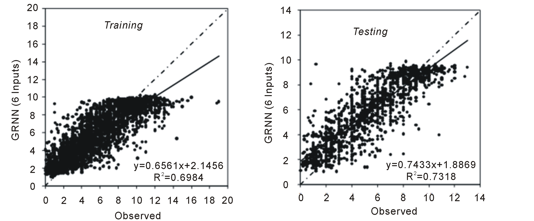
Figure 3. Scattering diagrams between GRSA results and observed pan evaporations (mm/day) during training and testing periods.
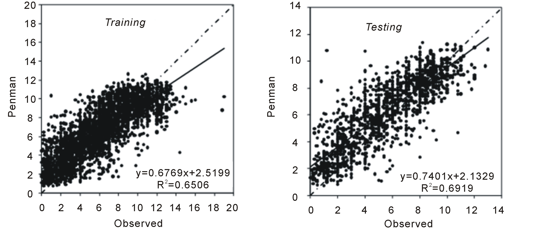
Figure 4. Scattering diagrams between Penman results and observed pan evaporations (mm/day) during training and testing periods.
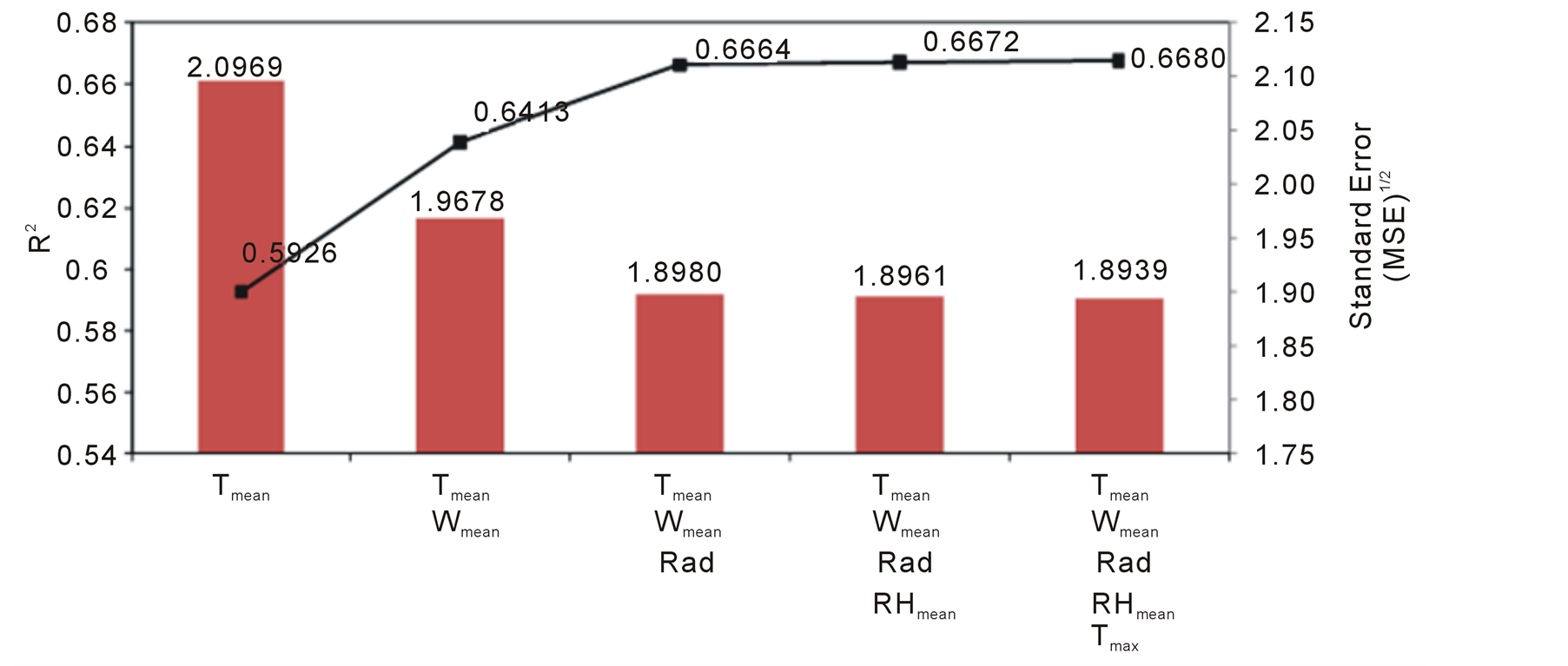
Figure 5. R2 and SE values of alternative regression models.
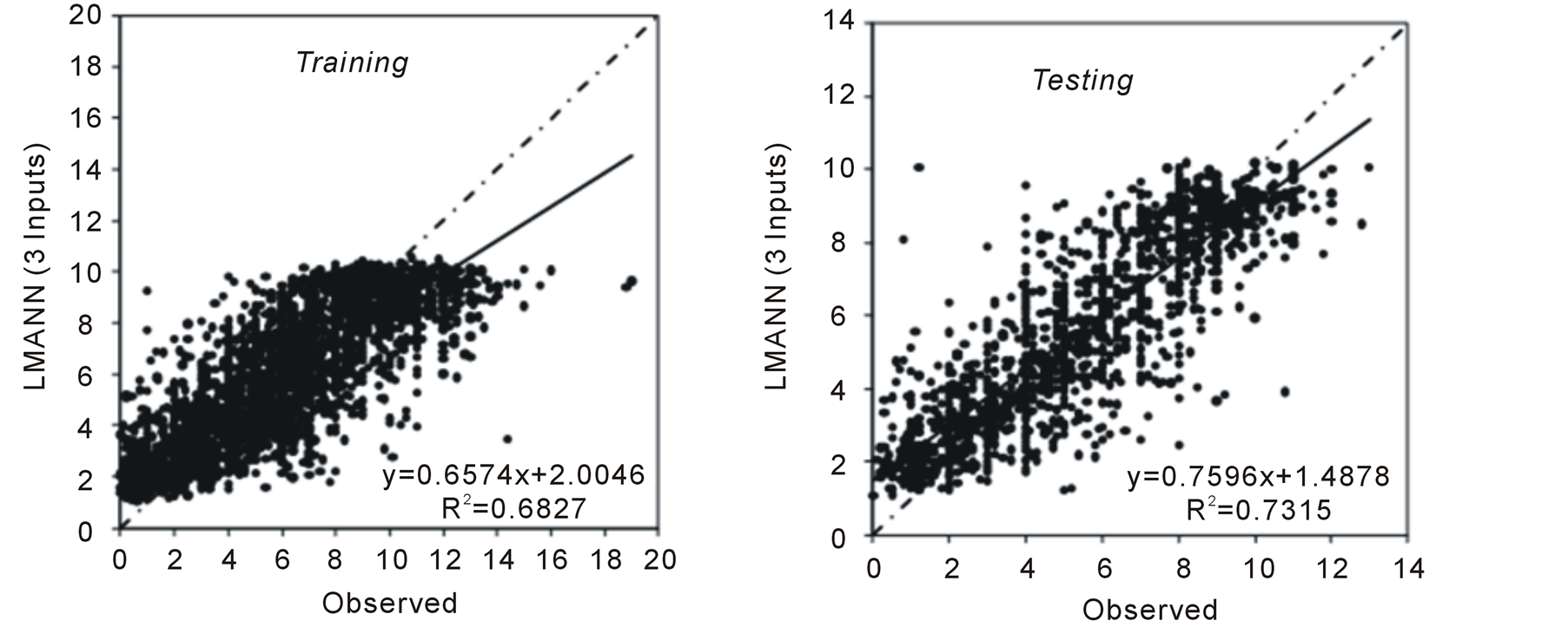
Figure 6. Scattering diagrams between LMANN with 3-inputs and observed pan evaporations (mm/day) during training and testing periods.
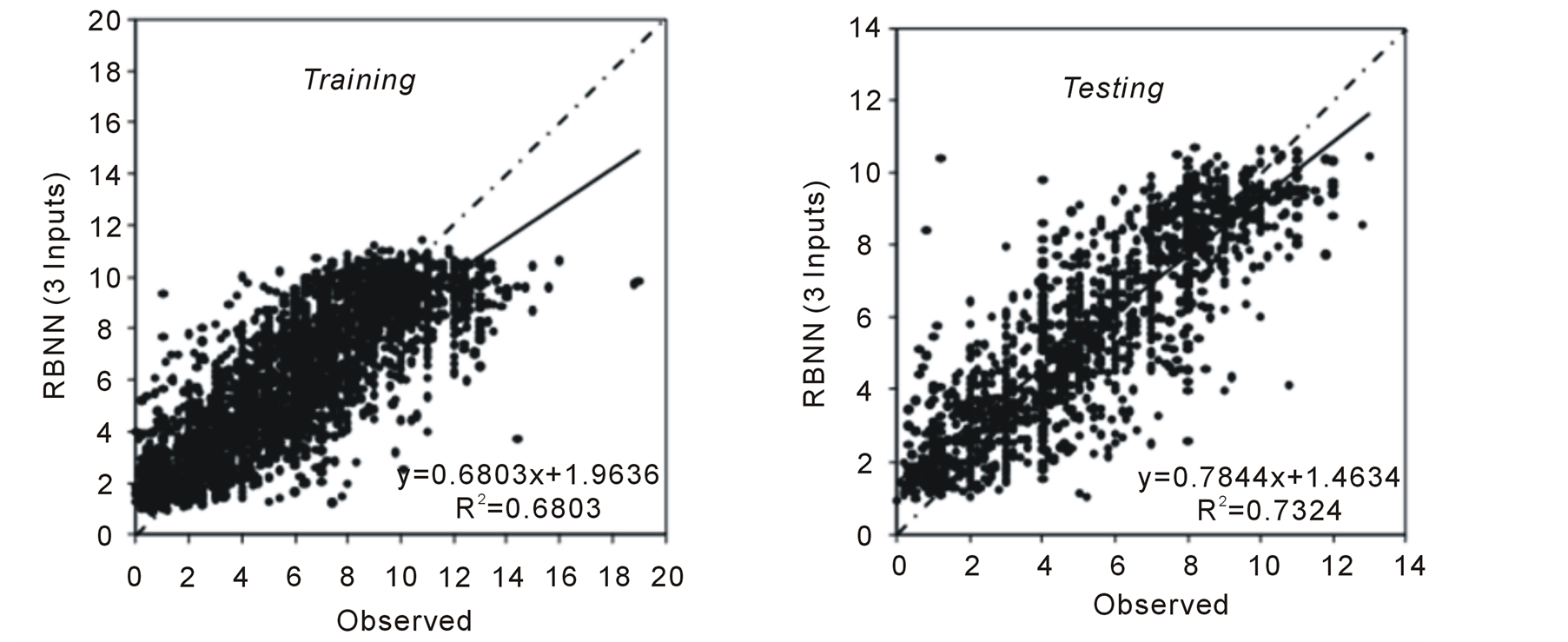
Figure 7. Scattering diagrams between RBANN results with 3-inputs for the periods of training and testing of observed pan evaporations (mm/day).
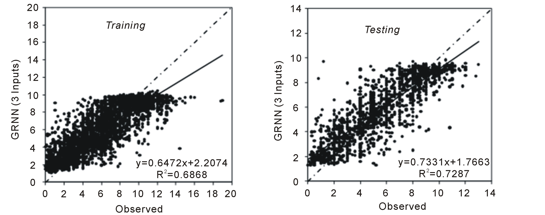
Figure 8. Scattering diagrams between GRNN with 3 inputs for the periods of training and testing and observed pan evaporations (mm/day).

Table 1. Comparison of basic statistics relevant models.
of mean square errors and basic statistics. Because of higher correlation with each other of certain parameters used in Penman equation (i.e., Tmax and Tmean), the number of inputs have been diminished with stepwise regression and, error performances of 3-inputs models during testing period has been found more effective. This situa
Table 2. Comparison of R2, MSE (mean of squared error) and error values of the models.
tion is worth considering the modeling studies in the regions and basins of no or insufficient daily evaporation data.
Models may be utilized mainly in winter seasons by the completion studies of missing pan evaporation data. The completed evaporation data by filling process may be also beneficial for the inputs of daily parametric models of water budget and also usable on stream basins as well as on reservoir basins of neighborhood dams.
On the farseeing directions under climate change, in the regions of either non-existed or insufficiently observed pan evaporation data depending on the increase of temperature and decrease of precipitation has also great importance. So, the computation of pan evaporation data will be then realized at the scenario-based critics.
References
- Kumar, M., Raghuwanshi, S., Singh, R., Wallender, W.W. and Pruitt, W.O. (2002) Estimating Evapotranspiration Using Artificial Neural Network. Journal of Irrigation and Drainage Engineering, 128, 224-233. http://dx.doi.org/10.1061/(ASCE)0733-9437(2002)128:4(224)
- Chauhan, S. and Shrivastava, R.K. (2009) Performance Evaluation of Reference Evapotranspiration Estimation Using Climate Based Methods and Artificial Neural Networks. Water Resources Management, 23, 825-837.
- Kim, S. and Kim, S.H. (2008) Neural Networks and Genetic Algorithm Approach for Nonlinear Evaporation and Evapotranspiration Modeling. Journal of Hydrology, 351, 299-317. http://dx.doi.org/10.1016/j.jhydrol.2007.12.014
- Piri, J., Amin, S., Moghaddam, A., Keshavarz, A., Han, D. and Remesan, R. (2009) Daily Pan Evaporation Modeling in a Hot and Dry Climate. Journal of Hydrologic Engineering, 803-811. http://dx.doi.org/10.1061/(ASCE)HE.1943-5584.0000056
- Trajkovic, S., Todorovic, B. and Stankovic, M. (2003) Forecasting Reference Evapotranspiration by Artificial Neural Networks. Journal of Irrigation and Drainage Engineering, ASCE, 129, 454-457. http://dx.doi.org/10.1061/(ASCE)0733-9437(2003)129:6(454)
- Whitley, R., Medlyn, B., Zeppel, M., Macinnis-Ng, C. and Eamus, D. (2009) Comparing the Penman-Monteith Equation and a Modified Jarvis-Stewart Model with an Artificial Neural Network to Estimate Stand-Scale Transpiration and Canopy Conductance. Journal of Hydrology, 373, 256-266. http://dx.doi.org/10.1016/j.jhydrol.2009.04.036
- Terzi, Ö. and Keskin, E. (2010) Comparison of Artificial Neural Networks and Empirical Equations to Estimate Daily Pan Evaporation. Journal of Irrigation and Drainage Engineering, 59, 215-225.
- Moghaddamnia, A., Gousheh, M.G., Piri, J., Amin, S. and Han, D. (2009) Evaporation Estimation Using Artificial Neural Networks and Adaptive Neuro-Fuzzy Inference System Techniques. Advances in Water Resources, 32, 88-97. http://dx.doi.org/10.1016/j.advwatres.2008.10.005
- Chang, F.J., Chang, L.C., Kao, H.S. and Wu, G.R. (2010) Assessing the Effort of Meteorological Variables for Evaporation Estimation by Self-Organizing Map Neural Network. Journal of Hydrology, 384, 118-129. http://dx.doi.org/10.1016/j.jhydrol.2010.01.016
- Abtew, W. (2001) Evaporation Estimation for Lake Okeechobee in South Florida. Journal of Irrigation and Drainage Engineering, 127, 140-147. http://dx.doi.org/10.1061/(ASCE)0733-9437(2001)127:3(140)
- Penman, H.L. (1948) Natural Evaporation from Open Water, Bare Soil and Grass. Proceedings of the Royal Society London A, 194, 120-145. http://dx.doi.org/10.1098/rspa.1948.0037
- Ham, F. and Kostanic, I. (2001) Principles of Neuro Computing for Science and Engineering. MacGraw-Hill, New York.
- Hagan, M.T. and Menhaj, M.B. (1994) Training Feed forward Techniques with the Marquardt Algorithm. IEEE Transactions on Neural Networks, 5, 989-993. http://dx.doi.org/10.1109/72.329697
- Broomhead, D.S. and Lowe, D. (1988) Multivariate Functional Interpolation and Adaptive Network. Complex Systems 2, 321-355.
- Specht, D.F. (1991) A General Regression Neural Network. IEEE Transactions Neural Network, 2, 568-576. http://dx.doi.org/10.1109/72.97934
- Okkan, U., Şerbeş, Z. and Dalkılıç, H.Y. (2011). Yapay Sinir Ağları ve Ampirik Yöntemlerle Balık Tava Buharlaşmalarının Tahmini (In Turkish, Estimation of fish-pan evaporations with the help of ANN and empirical methods). Ankara, DSİ Teknik Bülteni (Technical Bulletin of State Water Authority), #111.
NOTES

*Corresponding author.