ABSTRACT

This paper made a discuss on the relative efficiency of the generalized conditional root square estimation and the specific conditional root square estimation in paper [1,2] in inhomogeneous equality restricted linear model. It is shown that the generalized conditional root squares estimation has not smaller the relative efficiency than the specific conditional root square estimation, by a constraint condition in root squares parameter, we compare bounds of them, thus, choose appropriate squares parameter, the generalized conditional root square estimation has the good performance on mean squares error.

1. Definition and Lemma

Definition 1 [1] In the model (1), defined as is the specific conditional root square estimation of:

where 0 < k < 1,

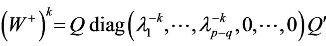, W, V defined as above paper, Q is p-orthogonal matrix, make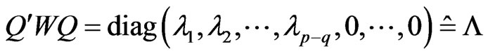, is Non-zero characteristic values of W, and .

Definition 2 [2] In the model (1), defined as is the generalized conditional root square estimation of:

.

where,

.

said is -root square parameter, W, Q, V defined as above paper.

Definition 3 [3] Two estimation and of the model (1), defined as is elative efficiency of estimation for elative efficiency estimation of. If is the best linear unbiased estimation of, then note.

For the above definition 3, if, then shows that is better than under mean squares error and if the bigger of (that efficiency highter), improve the degree of bigger.

Lemma 1 [1],.

Lemma 2 [1] 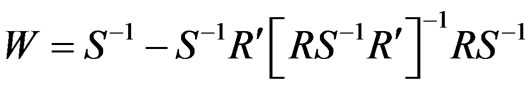is positive semidefinite matrix, and rank of W is.

Lemma 3 [1] Exist Q is p-order orthogonal matrix,

make, is Non-zero characteristic values of W, and .

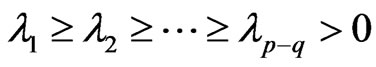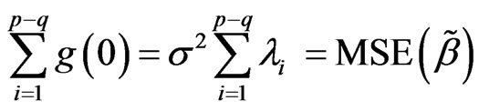
Lemma 4 [1] Mean squares error of is

, is Non-zero characteristic values of W, and.

Lemma 5 [1] Assume 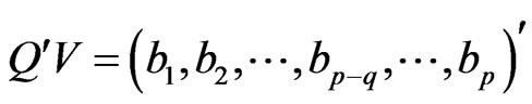then

where.

2. Main Results

We can prove the following exist theorem and bound of and. Now, we have the following lemma.

Assume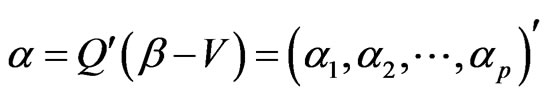, then .

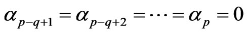And the RLSE of is

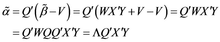
accordingly, the specific conditional root square estimation of is

0 < k < 1.

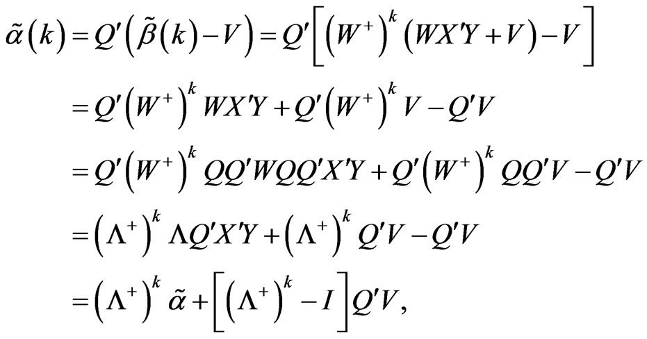
similarly, the generalized conditional root square estimation of is

.

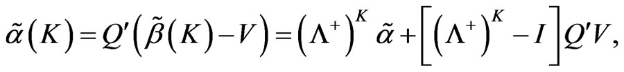
Lemma 6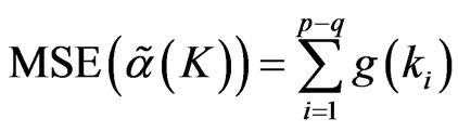, where .

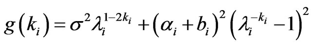Proof:

when,.

Because,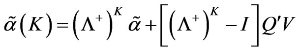

so .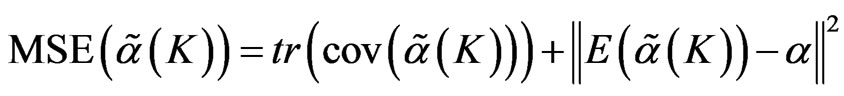

Because

So

Lemma 7,

.

Lemma 8 When, exist, when, then

has minimum value.

Proof: Note, , then.

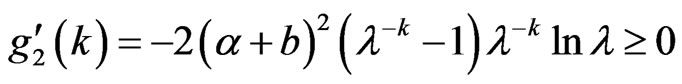
For, we have. When, if, then,; if, then,. When,. so is a monotonically decreasing function in.

For, when, we have

. this means

is a monotonically increasing function in. so, there always exist, whenwe have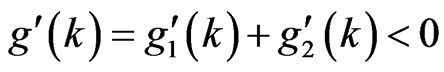, so is a monotonically decreasing function in, <, has minimum value.

Lemma 9 In the model (1), for

, when , then has minimum value.

Proof: according to lemma 8,

Let, we get

when, the solution of this equation is; when, the solution of this equation is

, that.

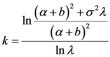so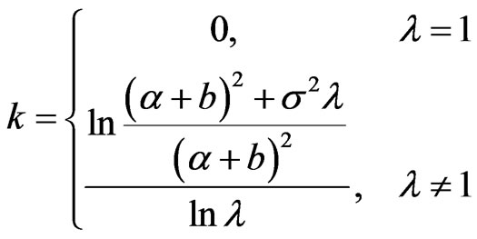. Therefore when , then has minimum value.

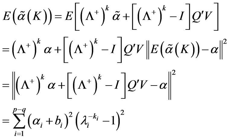
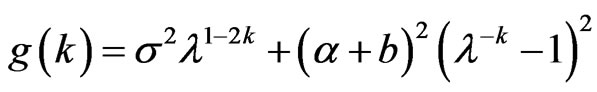
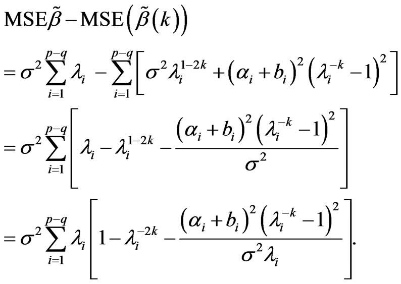
Lemma 10 In the model (1), exist root square parameter 0 < k < 1, then mean squares error of is

.

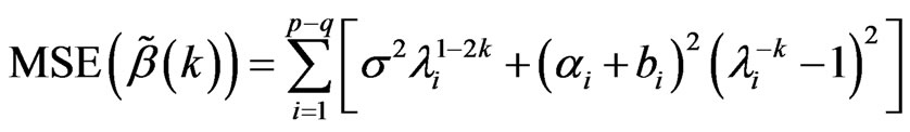Lemma 11 In the model (1), 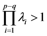, always exist, then.

Proof: Based on the lemma 9 and lemma 10.

Theorem 1 In the model (1), , always exist, then.

Proof: Based lemma 11 and definition 3, we get the conclusion.

Theorem 2 In the model (1), for, exist, then.

Proof: For, if, , choose,

we have .

Assume at least exist i, that, assume, where , based on lemma 6 and, we have

based on lemma 9, we have, then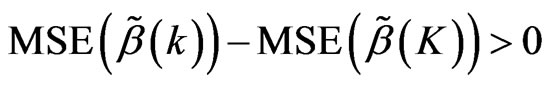, so .

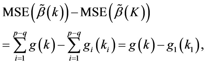
For above theorem, then.

Using theorem 2, we get the following the conclusion.

Inference 1 In the model (1), for, exist,

then.

Inference 2 In the model (1), if Are not all equal,

then.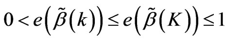

Proof: Because, Q is orthogonal matrix, so when, then, based on theorem 2, we get the conclusion.

Theorem 3 In the model (1), when

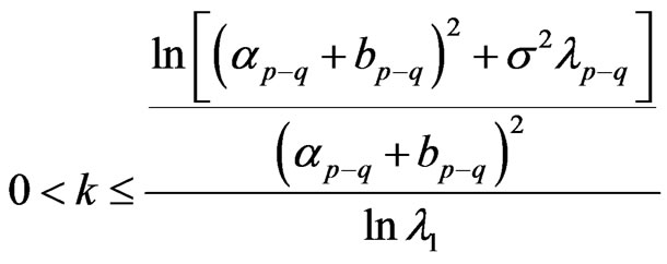then, where

,

is 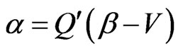the largest component of module.

Proof: Assume, then

Assume

then

so.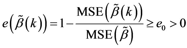

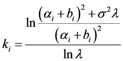
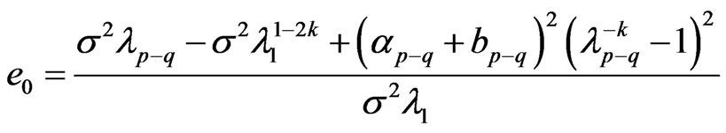
Theorem 4 In the model (1), for, if , , then, Where

.

Proof:

Therefore, let,

then.

Theorem 5 In the model (1), assume the non-zero characteristic root of W are not all equal , for the efficiency lower bound of and the efficiency lower bound of, the relationship of them is.

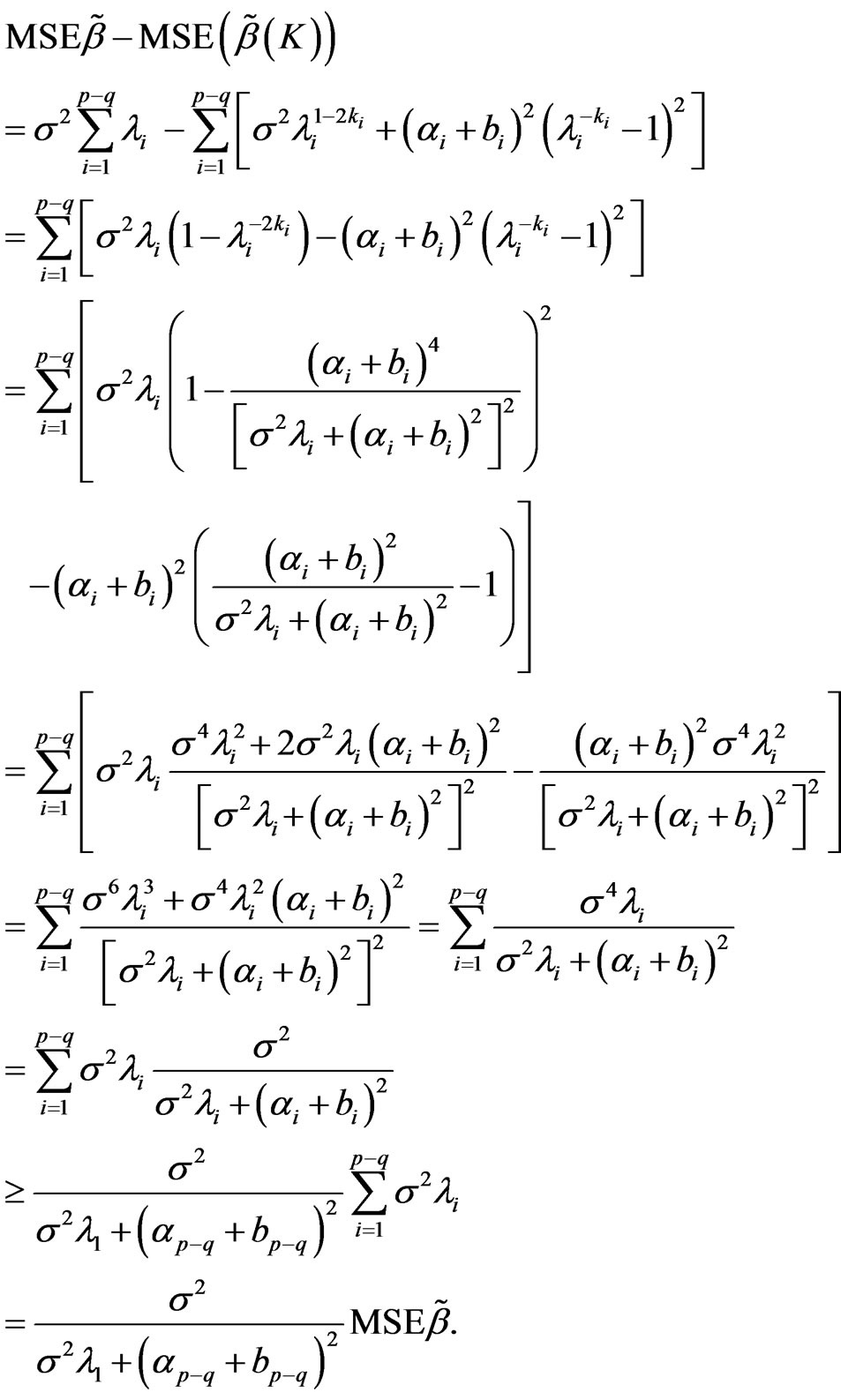
Proof: By theorems 3 and 4, we get ,

note then

,

Then

As are not all equal, therefore, also, then, thus.

That.

REFERENCES

- X.-L. Nong and W.-R. Liu, “The Conditional Root Square Estimation of Parameter of Restricted Linear Model,” Journal of Chongqing Normal University (Natural Science Edition), No. 2, 2007, pp. 24-28.
- X.-L. Nong, W.-R. Liu, et al., “The Generalized Conditional Root Squares Estimation of Parameter in Restricted Linear Model,” Journal of Guangxi University of Technology, Vol. 18, No. 3, 2007, pp. 24-27.
- P.-H. Wang, “The Relative Efficiency of the Generalized Ridge Estimation,” Journal of QuanZhou Normal College, Vol. 2, 1998, pp. 13-15.