Intelligent Control and Automation
Vol.4 No.3(2013), Article ID:35649,8 pages DOI:10.4236/ica.2013.43038
Slip Suppression of Electric Vehicles Using Sliding Mode Control Method*
1Department of Computer Science, University of Tsukuba, Tsukuba, Japan
2Faculty of Engineering, Information and Systems, University of Tsukuba, Tsukuba, Japan
Email: li@acs.cs.tsukuba.ac.jp, kawabe@cs.tsukuba.ac.jp
Copyright © 2013 Shaobo Li, Tohru Kawabe. This is an open access article distributed under the Creative Commons Attribution License, which permits unrestricted use, distribution, and reproduction in any medium, provided the original work is properly cited.
Received February 4, 2013; revised March 4, 2013; accepted March 11, 2013
Keywords: Sliding Mode Control; Slip Ratio; Electric Vehicles; Robustness; Energy Conservation
ABSTRACT
This paper presents a slip suppression controller using sliding mode control method for electric vehicles which aims to improve the control performance and the energy conservation by controlling the slip ratio of wheel. In this method, a robust sliding mode controller against the model uncertainties is designed to obtain the maximum driving force by suppressing the slip ratio. The numerical simulations for one wheel model under variations in mass of vehicle and road condition are performed and demonstrated to show the effectiveness of the proposed method.
1. Introduction
In recent years, as a powerful solution against the environment and energy problems, Electric Vehicles (EVs) have attracted great interests in the world [1]. Compared with Internal Combustion Engine Vehicles (ICEVs), on one hand, EV is more environmental-friendly vehicle. On the other hand, it has significant performance advantages from the standpoint of electric and control engineering as the torque response is very quick and the torque can be measured easily and accurately [2]. As a result, advanced motion control such as the traction control with wheel slip suppression can be realized more easily for EVs than ICEVs [3,4].
As known to all, it is important to have good energy conservation for EVs, so it is hoped that there will be a control method which can reduce the electric energy consumption. When the vehicle is starting off or accelerating under slippery road conditions, the driving wheels falling into slip easily causes unstable driving situation and a lot of energy waste. The traction control is to provide the maximum driving force for driving wheels when accelerating, especially in wet, icy or snowy road conditions. For improving acceleration performance and saving electric energy for EVs, an advanced traction control is expected. During acceleration, the driving force of wheel directly depends on the friction coefficient between road and tire, which is in accordance with the wheel slip and road conditions. For this reason, it becomes possible to influence driving force by controlling the wheel slip.
There have been several methods proposed for the slip control of EVs, such as the method based on Model Following Control (MFC) in [5] and Model Predictive PID method (MP-PID) in [6]. Both of these methods show good performances under the nominal conditions where the situations, for example, mass of vehicle, road condition, and so on, are not changed. To meet high performance to the variation happened in these conditions, it is significant to construct robust control systems against the situation changing. About this point, Sliding Mode Control (SMC) has been performed good robustness for the systems with uncertainties and nonlinearities. Thereby [7,8] introduced robust control methods based on SMC for anti-lock braking system.
In SMC, system trajectory is forced to reach the desired geometrical locus called sliding surface, then the trajectory slides along it when the motion of the system is in sliding mode [9,10]. The control objective of SMC is to take the system trajectory to reach the sliding surface in finite time, then to behave in sliding mode. In original SMC, chattering phenomenon always occurs through switching of the control inputs due to the variable structure of the sliding mode controller [11]. For reducing such undesired chattering effect, normally one boundary layer around the sliding surface is introduced in [12]. In contrast, the control performance such as steady state accuracy and transient response performance gets degradation, and moreover, it leads to energy loss. To overcome these disadvantages of conventional SMC method, an integral term is introduced in the design of the sliding surface [13]. Moreover, in order to get better control performance and save more energy, a new robust control method based on SMC for slip suppression of EVs is proposed. The numerical simulation results show the effectiveness of the proposed method.
2. Preliminaries of SMC
Consider a single input nonlinear dynamical system [12] described by
 (1)
(1)
where  is the state vector and
![]() is the control input. In general, the function
is the control input. In general, the function  and the control gain
  are not exactly known but the extents of the imprecision on
  and
and  are upper bounded by known. The control problem is to seek a solution that is robust to uncertainties in
  and
and . Firstly, we defined a time-varying surface
  in the state space
  by
by
 (2)
(2)
where  is the error between the output state
 ![]() and the desired state
and the desired state . The problem of tracking
  is equivalent to remaining on the surface
 ![]() for all
for all . When
 , that is to say, the system trajectory reaches the surface which represents the error is zero. Hence,
  describes the sliding surface where the error will converge to zero exponentially. When
 , the trajectory is restricted to the sliding surface, which represents that the motion of the system is in sliding mode.
The SMC law contains two parts, the equivalent control input  and the hitting control input
 , which is defined as follows,
 (3)
(3)
 can be interpreted as the continuous control law which would maintain
  when the dynamics is exactly known. When the dynamics is not exactly known, such as the uncertainties occur in the system or the trajectory of system is off the sliding surface,
  acts to bring the trajectory back to the sliding surface and keeps it in sliding mode. Generally,
  uses a discontinuous function to implement the switching action on sliding surface.
For choosing the control input![]() , it is necessary to consider the sliding condition [12], which is defined as
, it is necessary to consider the sliding condition [12], which is defined as
 (4)
(4)
where . From Equation (4),
  shows that the squared distance to the sliding surface, which decreases along all system trajectories. Particularly, once the system trajectories reach the surface, they will remain on the surface. In other words, the system satisfying the sliding condition makes the trajectories reach the surface in finite time, and once on the surface, they cannot leave it. Furthermore, Equation (4) also implies that some dynamic uncertainties can be tolerated by keeping the motion of the system in sliding mode.
In general, to design a control system based on SMC should go through the following two steps. Firstly, design a sliding surface ![]() which is invariant of the controlled dynamics. Secondly, choose the control input
which is invariant of the controlled dynamics. Secondly, choose the control input ![]() which drives the system trajectory to the sliding surface in sliding mode in finite time.
which drives the system trajectory to the sliding surface in sliding mode in finite time.
3. Problem Formulation
3.1. Vehicle Dynamics
A vehicle model which is appropriate for acceleration on the longitudinal direction is described here. For simplicity, one wheel model directly driven by an electric motor is used for the derivation of control law and numerical simulations. Although the one wheel model is quite simple, it still retains the essential dynamics of the system. In deriving the dynamic equations of the system, the lateral and vertical motions are neglected. The rolling resistance and air resistance are also ignored. A simple one wheel model is shown in Figure 1.
The dynamic equation for the wheel rotating motion and longitudinal vehicle motion are given by
 (5)
(5)
 (6)
(6)
 (7)
(7)
where ![]() is the angular velocity of wheel,
is the angular velocity of wheel,  the radius of wheel and V the vehicle body speed. Other parameters are defined in Table 1.
The tire driving force  is given by
 (8)
(8)
where  is the friction coefficient as hereinafter defined and the normal tire force
  is defined as
 (9)
(9)
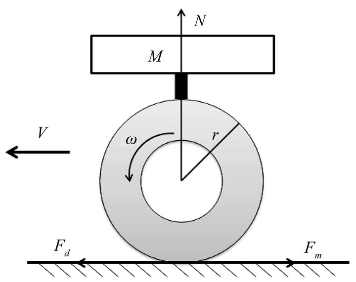
Figure 1. One wheel model of cars.
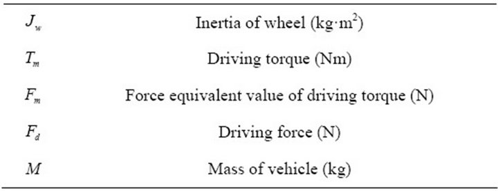
Table 1. Vehicle model parameters.
where ![]() is the acceleration of gravity.
is the acceleration of gravity.
The friction coefficient , which is the ratio between the driving force and the normal tire force, depends on the road condition (represented by road surface condition coefficient
![]() ) and the wheel slip (represented by slip ratio
) and the wheel slip (represented by slip ratio![]() ). The slip ratio is defined as
). The slip ratio is defined as
 (10)
(10)
where  is wheel speed. The slip ratio of
  characterizes the wheel is completely skidding. If the slip ratio gets the value
 , no skidding is happening at the point of contact of tire with road.
The friction coefficient  is a function of road surface condition coefficient
 ![]() and slip ratio
and slip ratio![]() , which is called Magic-Formula and given in [14] by
, which is called Magic-Formula and given in [14] by
 (11)
(11)
Figure 2 shows the relationship between friction coefficient  and slip ratio
 ![]() on the road surface conditions for dry asphalt
on the road surface conditions for dry asphalt , wet asphalt
  and ice road
 . It also represents how the friction coefficient
  increases with slip ratio
 ![]() up to a value
up to a value 
 where it obtains the maximum value of friction coefficient. As defined in Equation (8), the driving force also reaches the maximum value corresponding to the friction coefficient. However, for satisfying
 , the friction coefficient decreases to the minimum value where the wheel is completely skidding. In consequence, to obtain the maximum value of driving force, it is expected to control the slip ratio ap-
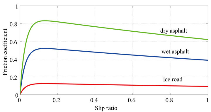
Figure 2. Relationship between slip ratio and friction coefficient.
proximately .
.
3.2. Derivation of Reference Slip Ratio λ*
Let us choose the function  defined as
 (12)
(12)
By using Equation (12), Equation (11) can be rewritten as
 (13)
(13)
From Figure 2, evaluating the values of ![]() which maximize
which maximize  for different
  means to find the value of
 ![]() where the maximum value of the function
where the maximum value of the function  can be obtained. Let
 (14)
(14)
and solving Equation (14) gives
 (15)
(15)
 (16)
(16)
Accordingly, for different road conditions, when  is met, the maximum driving force can be achieved. In this paper, the value of reference slip ratio
  is set to 0.13.
To obtain the maximum driving force all the time, the slip ratio needs to be kept at the reference value stably and accurately on any cases, but in fact the road surface on which vehicles travel is not at a constant condition always. Besides, the mass of vehicle varies when the weight of load such as the luggage and passengers changes. Consequently, we need to control the slip ratio under the condition of the often change of vehicle mass and road condition.
3.3. Evaluation of Electric Energy Consumption
In this paper, we estimate the energy cost of EVs by calculating the electric energy consumed by motor. At first, we make the following assumptions. Assumption 1, the electric energy consumed by motor is all used to drive the wheel. Assumption 2, the energy consumed is equal to the work of motor. Then, the total electric energy consumed  can be written by the driving torque of motor
  and the angle of rotation
  as
as
 (17)
(17)
4. SMC with Integral Action for Slip Ratio Control
For slip ratio control, a nonlinear controller using SMC with integral action is proposed. Without loss of generality, the control law is derived based on the one wheel model mentioned above. The system dynamics can be written as
 (18)
(18)
where  is the state of system representing the slip ratio of driving wheel which is defined as Equation (10) in situation of acceleration.
  is the control input.
Differentiating Equation (10) with respect to time
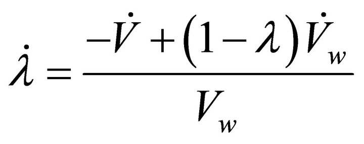 (19)
(19)
And substituting Equations (5), (6) and (8) into Equation (19), the following equations can be obtained,
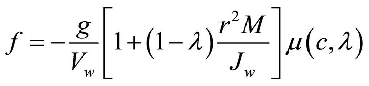 (20)
(20)
 (21)
(21)
The control objective is to control the value of the slip ratio to the constant reference value .
.
Actually, the mass of vehicle often changes with the number of passengers and the weight of luggage. Besides, the vehicle always travels on various kinds of road surfaces. As a result, the controller needs to perform much robustly with the uncertainties affecting on the mass of vehicle and road surface condition which are represented by  and
and ![]() respectively. The ranges of variation in
respectively. The ranges of variation in  and
and ![]() are set as
are set as
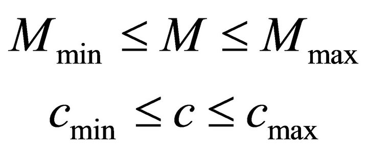 (22)
(22)
Consider the system Equation (18), the nonlinear function  is not exactly known, but it can be estimated as
 . The estimation error on f is assumed to be bounded by a known function
 ,
,
 (23)
(23)
The uncertainty in f is due to the parameter M and c. Accordingly, by using Equation (20) the estimation of f can be defined as
 (24)
(24)
where  is the estimated value of M and
  is estimated for c.
Here, we define the estimated values of these parameters respectively by using the arithmetic mean of the value of the bounds as
 (25)
(25)
From these definitions, the error in estimation can be given by
 (26)
(26)
Then, we let
 (27)
(27)
4.1. Design of Sliding Surface
Letting ![]() be the variable of interest, then the order of system is assumed to be one. The sliding function of conventional SMC can be given by
be the variable of interest, then the order of system is assumed to be one. The sliding function of conventional SMC can be given by
 (28)
(28)
where ![]() is the error between the actual slip ratio and the reference value, which is defined as
is the error between the actual slip ratio and the reference value, which is defined as .
.
By adding an integral item to the sliding function , the new sliding function
  can be written as
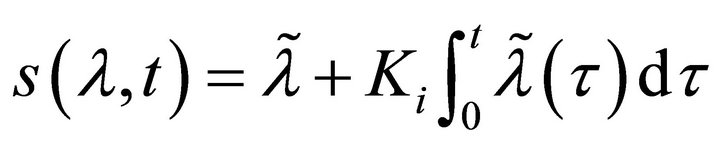 (29)
(29)
where  is the integral gain,
4.2. Derivation of Control Law
In this section, the sliding mode controller is derived to make the slip ratio ![]() converge to the reference value
converge to the reference value . The sliding mode happens when the trajectory reaches the sliding surface defined by
 . The dynamics of sliding mode is governed by
 (30)
(30)
Differentiating Equation (29), then substituting the result into Equation (30) gives
 (31)
(31)
The reference slip ratio λ* is a constant, thus . Substituting Equation (18) into Equation (31) gives
 (32)
(32)
and solving Equation (32) gives equivalent control input as
 (33)
(33)
Then the estimate of the equivalent control input can be obtained as
 (34)
(34)
For meeting the sliding condition (making the system trajectory in the sliding mode) despite uncertainties on the dynamics f, the hitting control input is defined as
 (35)
(35)
where
 (36)
(36)
and  is called sliding gain. Thus, the control law can be given by
 (37)
(37)
When there is no uncertainty existing in the system dynamics (i.e., no variation in c and M),  is desired to be 0. Because Equation (37) contains the estimate of the equivalent control
 ,
,  keeps the trajectory on the sliding surface (
 , i.e.,
 ). Because of the uncertainties, the trajectory deviates from the sliding surface. The hitting control acts to return the trajectory back to the sliding surface which implies the robustness of SMC.
Here, the sliding gain  is chosen as
 (38)
(38)
with the value of  given by Equation (27).
  is a design parameter described in Equation (4), which is a strictly positive constant.
Then choose a Lyapunov function as
 (39)
(39)
and differentiate Equation (39) with respect to time, that gives
 (40)
(40)
Substituting Equations (18), (30), (34), (35) and (37) into Equation (40) yields
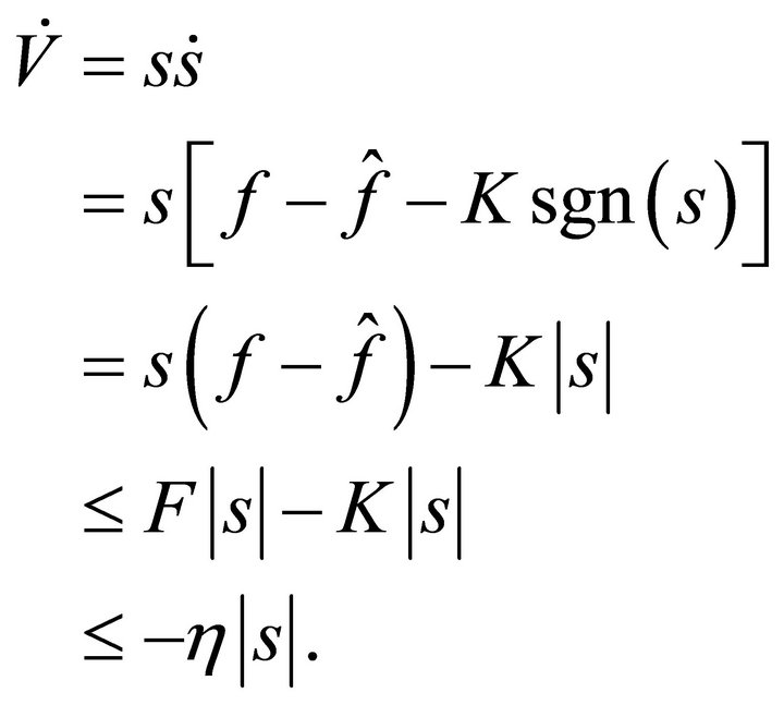 (41)
(41)
Thus, the control law introduced in Equation (37) can guarantee the stability of the system in the Lyapunov sense under variations. Concretely, the stability of the system is guaranteed with an exponential convergence once the sliding surface is encountered, when the sliding condition is satisfied. So Equation (41) guarantees that the trajectory will converge to the sliding surface in finite time if the error is not zero. That is to say, slip ratio can be suppressed to the reference value in finite time whenever the uncertainties occur in the system.
4.3. Chattering Reduction
In design of sliding mode control system, the switched control law requires switching at an infinite frequency. However, because the actuators have time delays and other imperfections, the action can lead to chatter in a neighborhood of the sliding surface. To reduce the chattering, the hitting control  can be rewritten by using the saturation function
 (42)
(42)
where  is a design parameter representing the width of the boundary layer around the sliding surface
  and the saturation function is defined as
 (43)
(43)
Thus, by using Equations (37), (38) and (42), the control law of the system by the proposed SMC can be rewritten as
 (44)
(44)
5. Numerical Simulations
The numerical simulations have been done using MATLAB/Simulink software [15]. The computer platform is listed in Table 2.
The simulation conditions are described here. The simulation time is set to 10 (s) in all. There are three phases in the simulations as follows. The first phase, the time is from 0 (s) to 2 (s) and the car travels on the dry asphalt. The second phase, from 2 (s) to 8 (s), the car travels on ice road. The last phase, the car runs on wet asphalt during 8 (s) to 10 (s). The width of the boundary layer  defined in Equation (42) is set to 1. In Equation (44), the proposed SMC law can be calculated with the values of design parameters
  and
and , which both impact on the steady state accuracy. Here, in order to confirm the effectiveness for the energy conservation performance of the proposed method, the values of both parameters are chosen as
  and
and , which are determined by trial and error.
By using Equations (28), (30), (35) and (38), the control law of the conventional SMC can be derived as
 (45)
(45)
Likewise, in the conventional SMC, the parameters  and
and . The values of parameters used in the simulations are listed in Table 3.
As the input to the simulation of system, the torque is produced by the pressure on the accelerator pedal, which is decided on the car speed desired by the driver. Here, the car speed is desired to achieve 180 (km/h) in 15 (s) by a fixed acceleration after starting the car. The range of variation in mass of the car M and road condition coefficient c are imposed as  (kg),
(kg),  (kg),
(kg),  and
and  respectively. So the nominal values of mass and road condition coefficient
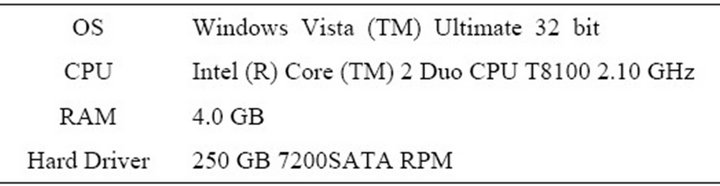
Table 2. Computer platform for the simulations.
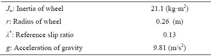
Table 3. Parameters used in the simulations.
can be obtained as 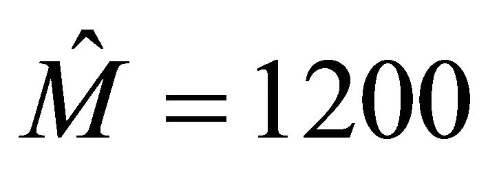 (kg) and
 .
.
5.1. Results of Robustness to the Variation in Mass and Road Condition
In order to verify the robustness of proposed SMC with variation both in the mass of the car and road condition, the variation in the mass of the car is made by assigning the value of  to 1000 (kg), 1100 (kg), 1200 (kg), 1300 (kg) and 1400 (kg) respectively. Figure 3 shows that the responses of slip ratio with different masses can converge to the reference value under the variation in the road condition. It is known that when the mass gets the nominal value 1200 (kg), in the first 2 (s), the response is more accurately than the car with other masses. But after 2 (s), the performance drops down with the mass increasing.
Next, we compare the proposed SMC with the conventional SMC and the case no control method used in the system.
Figures 4-8 show the responses of slip ratio under three different road conditions for five different masses respectively. The responses with proposed SMC can suppress the slip ratio to the reference value 0.13 accurately in a very short time whenever both of the mass and road condition are changing. In addition, the slip ratio with the conventional SMC does not converge to the reference value because of the steady state error. When the car starts off at 0 (s) or runs into an ice road at 2 (s), the slip ratio response using control method grows with the in-
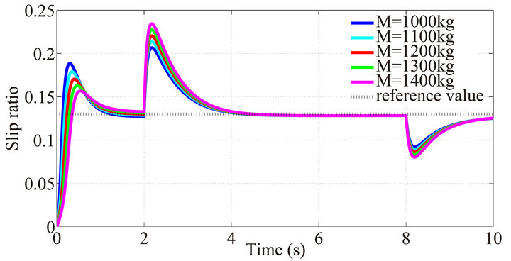
Figure 3. Slip ratio by using proposed SMC.
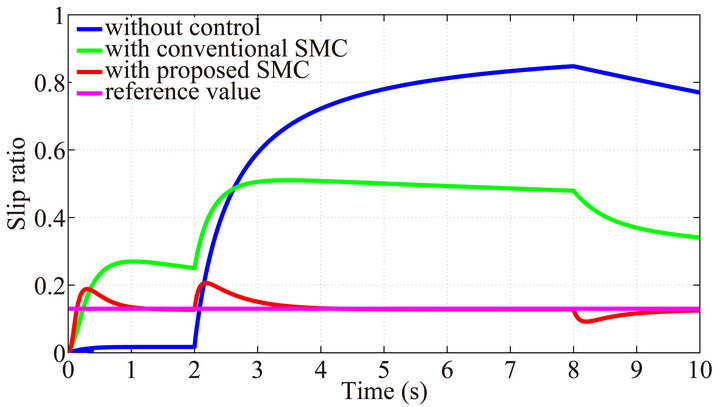
Figure 4. Slip ratio with mass of vehicle equals 1000 (kg).
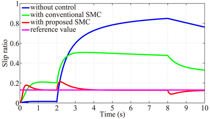
Figure 5. Slip ratio with mass of vehicle equals 1100 (kg).

Figure 6. Slip ratio with mass of vehicle equals 1200 (kg).

Figure 7. Slip ratio with mass of vehicle equals 1300 (kg).
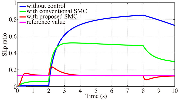
Figure 8. Slip ratio with mass of vehicle equals 1400 (kg).
creasing wheel speed as a result of too much torque generated. As the car travels from ice road to wet asphalt from 8 (s), the slip ratio decreases with the decreasing wheel speed, when the torque generated at that time cannot meet that required on the wet asphalt. The car without control is to make the slip ratio to 0, so at the first stage the response is converged to 0. However, when the car runs into the ice road at 2 (s), the wheel spins out of control resulting that the wheel speed increasing suddenly, which leads to a large slip ratio value. Therefore, we can see that the proposed SMC have a good performance against the variation in both of the mass of the car and road condition.
5.2. Results of Acceleration Performance
It is different from the simulation condition described in previous that the simulations are executed under unchanging road condition and mass every time. Figure 9 shows the time required for 100 meters by the car with different control method. The x-axis label indicates the cases of different road condition and mass, for example, DA1000 says that the car with the mass 1000 (kg) is driving on the dry asphalt, WA1200 shows that the case with the mass 1200 (kg) on the wet asphalt and IR1400 is the case with mass 1400 (kg) on the ice road. As shown in the bar graph, it takes the minimum time for the car with the proposed method for the 100 meters in every case. So we can see that the car with proposed SMC have gained the best acceleration. In other words, the results also indicate the car with the proposed SMC decreases the loss of driving force mostly. Moreover, the time required is long on the ice road because the car cannot get enough driving force to accelerate on the slippery road.
5.3. Results of Energy Conservation
To confirm the effectiveness of the proposed SMC for energy conservation, we compare it to the conventional SMC and no control method. As a numerical example, we calculate the energy consumed in the simulations executed in 5.1. Figure 10 shows the results of electric energy consumed by different mass cases.
We can see that the proposed SMC consumes the minimum energy in every case. The car without control takes most energy because the spin of wheel on the ice road from 2 (s) to 8 (s) leads to much energy loss. As the mass increases, the amount of energy cost decreases because the car suppresses the spin of wheel by increment
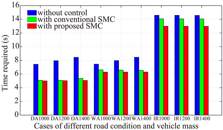
Figure 9. Time required for 100 (m).

Figure 10. Electric energy consumed by mass.
of mass to get more driving force. Conversely, the energy consumption with the proposed SMC and conventional SMC increases due to the rising cost of control as the mass increases. From this perspective, it also implies that an EV should be made more light to save more energy.
6. Conclusions
This paper proposed an extended SMC method adding the integral term to the sliding function for improving the performance of the slip ratio control for EVs. The control objective focused on suppressing the slip ratio to the reference value within the specified variation in mass of vehicle and road conditions which allowed the vehicle to get the maximum driving force and minimum energy cost during acceleration.
As numerical examples based on the one wheel model, the simulations using the proposed method were executed, and the robustness to the uncertainties caused in mass of vehicle and road conditions was verified. Besides, by comparing to conventional SMC and no control, the vehicle with proposed method performed best acceleration performance; moreover, the results also showed that the proposed method could reduce the energy cost when the vehicle travels on a slippery road.
In our research, the design parameter  and the gain
  of integral item added in the sliding function was determined by trial and error, so it is necessary to develop a method to find the optimal value of
  and gain
 . Moreover, although the effectiveness of the proposed method for traction was just verified in the acceleration situation in this paper, we need to verify and improve the method for overall driving condition including braking situation. Then, the method is expected to be implemented and be one of the advanced motion control of EVs.
REFERENCES
- S. Brown, D. Pyke and P. Steenhof, “Electric Vehicles: The Role and Importance of Standards in an Emerging Market,” Energy Policy, Vol. 38, No. 7, 2010, pp. 3797- 3806. doi:10.1016/j.enpol.2010.02.059
- T. Hirota, M. Ueda and T. Futami, “Activities of Electric Vehicles and Prospect for Future Mobility,” Journal of the Society of Instrument and Control Engineers, Vol. 50, No. 3, 2011, pp. 165-170.
- T. Sakai and Y. Hori, “Advanced Vehicle Motion Control of Electric Vehicle Base on the Fast Motor Torque Response,” Proceedings of the 5th Annual International Symposium on Advanced Vehicle Control, Michigan, 2000, pp. 729-736.
- R. Shitato, T. Akiba, T. Fujita and S. Shimodaira, “A Study of Novel Traction Control Method for Electric Propulsion Vehicle,” Journal of the Society of Instrument and Control Engineers, Vol. 50, No. 3, 2011, pp. 195- 200.
- Y. Hori, “Simulation of MFC-Based Adhesion Control of 4WD Electric Vehicle,” Papers of Technical Meeting on Industrial Instrumentation and Control, Vol. 2C-00, No. 1-23, 2000, pp. 291-293.
- T. Kawabe, Y. Kogure, K. Nakamura, K. Morikawa and T. Arikawa, “Traction Control of Electric Vehicle by Model Predictive PID Controller,” Transaction of Japan Society of Mechanical Engineers, Series C, Vol. 77, No. 781, 2011, pp. 3375-3385. doi:10.1299/kikaic.77.3375
- C. Unsal and P. Kachroo, “Sliding Mode Measurement Feedback Control for Antilock Braking Systems,” IEEE Transaction on Control Systems Technology, Vol. 7, No. 2, 1999, pp. 271-281. doi:10.1109/87.748153
- M. Oudghiri, M. Chadli and A. E. Hajjaji, “Robust Fuzzy Sliding Mode Control for Antilock Braking Systems,” International Journal on Sciences and Techniques of Automatic Control, Vol. 1, No. 1, 2007, pp. 13-28.
- V. Utkin, J. Guldner and J. Shi, “Sliding Mode Control in Electro-Mechanical System,” 2nd Edition, Taylor & Francis Group, Boca Raton, 2009.
- K. Nonami and H. Tian, “Sliding Mode Control,” CORONA, Tokyo, 2000.
- J. Y. Hung, W. Gao and J. C. Hung, “Variable structure Control: A Survey,” IEEE Transaction on Industrial Electronics, Vol. 40, No. 1, 1993, pp. 2-22.
- J. J. E. Slotine and W. Li, “Applied Nonlinear Control,” Prentice-Hall, Inc., New Jersey, 1991.
- I. Eker and A. AKinal, “Sliding Mode Control with Integral Augmented Sliding Surface: Design and Experimental Application to an Electromechanical System,” Electrical Engineering, Vol. 90, No. 3, 2008, pp. 189-197. doi:10.1007/s00202-007-0073-3
- H. B. Pecejka and E. Bakker, “The Magic Formula Tyre Model,” Proceedings of the 1st International Colloquium on Tyre Models for Vehicle Dynamics Analysis, Vol. 21, Suppl. 001, 1991, pp. 1-18.
- The MathWorks, Inc., “MATLAB and Simulink Student Version,” 2011. http://www.mathworks.co.jp/academia
NOTES
*This research was partially supported by Grant-in-Aid for Scientific Research (C) (Grant number: 24560538; Tohru Kawabe; 2012-2014) from the Ministry of Education, Culture, Sports, Science and Technology of Japan.