Intelligent Control and Automation
Vol. 3 No. 4 (2012) , Article ID: 24881 , 14 pages DOI:10.4236/ica.2012.34042
Linear Inferential Modeling: Theoretical Perspectives, Extensions, and Comparative Analysis
1Chemical Engineering Program, Texas A & M University, Doha, Qatar
2Electrical and Computer Engineering Program, Texas A & M University, Doha, Qatar
Email: *mohamed.nounou@qatar.tamu.edu
Received July 26, 2012; revised August 26, 2012; accepted September 4, 2012
Keywords: Inferential Modeling; Latent Variable Regression; Regularized Canonical Correlation Analysis; Distillation Columns
ABSTRACT
Inferential models are widely used in the chemical industry to infer key process variables, which are challenging or expensive to measure, from other more easily measured variables. The aim of this paper is three-fold: to present a theoretical review of some of the well known linear inferential modeling techniques, to enhance the predictive ability of the regularized canonical correlation analysis (RCCA) method, and finally to compare the performances of these techniques and highlight some of the practical issues that can affect their predictive abilities. The inferential modeling techniques considered in this study include full rank modeling techniques, such as ordinary least square (OLS) regression and ridge regression (RR), and latent variable regression (LVR) techniques, such as principal component regression (PCR), partial least squares (PLS) regression, and regularized canonical correlation analysis (RCCA). The theoretical analysis shows that the loading vectors used in LVR modeling can be computed by solving eigenvalue problems. Also, for the RCCA method, we show that by optimizing the regularization parameter, an improvement in prediction accuracy can be achieved over other modeling techniques. To illustrate the performances of all inferential modeling techniques, a comparative analysis was performed through two simulated examples, one using synthetic data and the other using simulated distillation column data. All techniques are optimized and compared by computing the cross validation mean square error using unseen testing data. The results of this comparative analysis show that scaling the data helps improve the performances of all modeling techniques, and that the LVR techniques outperform the full rank ones. One reason for this advantage is that the LVR techniques improve the conditioning of the model by discarding the latent variables (or principal components) with small eigenvalues, which also reduce the effect of the noise on the model prediction. The results also show that PCR and PLS have comparable performances, and that RCCA can provide an advantage by optimizing its regularization parameter.
1. Introduction
Models play an important role in various process operations, such as process control, monitoring, and optimization. In process control, where measuring the controlled variable (s) is difficult, it is usually relied on inferential models that can estimate the controlled variable (s) from other more easily measured variables. For example, the control of distillation column compositions requires the availability of inferential models that can accurately predict the compositions from other variables, such as temperature and pressure at different trays of the column. These inferential models are expected to provide accurate predictions of the output variables over a wide range of operating conditions. However, constructing such inferential models is usually associated with many challenges, which include accounting for the presence of measurement noise in the data and dealing with collinearity or redundancy among the variables.
Collinearity is common in inferential models since they usually involve a large number of variables. The presence of collinearity increases the variance of the estimated model parameters, and thus degrades the prediction accuracy of the estimated models. Over-parameterized models can fit the original data well, but they usually lead to poor predictions [1]. One simple approach for dealing with this problem is to select a subset of independent variables to be used in the model [2-4]. Other modeling techniques that deal with collinearity can be divided into two main categories: full rank models and reduced rank models (or latent variable regression models). Full rank models utilize regularization to improve the conditioning of the input covariance matrix [5-7], and include Ridge Regression (RR). RR reduces the variations in the model parameters by imposing a penalty on the L2 norm of their estimated values. RR also has a Bayesian interpretation, where the estimated model parameters are obtained by maximizing a posterior density in which the prior density function is a zero mean Gaussian distribution [8].
Latent variable regression (LVR) models, on the other hand, deal with collinearity by transforming the variables so that most of the data information is captured in a smaller number of variables that are used to construct the model. In other words, LVR models perform regression on a small number of latent variables that are linear combinations of the original variables. This generally results in well-conditioned models and good predictions [9]. LVR model estimation techniques include principal component regression (PCR) [5,10], partial least squares (PLS) [5,11,12], and regularized canonical correlation analysis (RCCA) [13-16]. PCR is performed in two main step: transform the input variables using principal component analysis (PCA), and then construct a simple model relating the input to the transformed inputs (principal components) using ordinary least squares (OLS). Thus, PCR completely ignores the output(s) when determining the principal components. Partial least squares (PLS), on the other hand, transforms the variables taking the input-output relationship into account by maximizing the covariance between the transformed inputs and outputs variables. Therefore, PLS has been widely used in practice, such as in the chemical industry to estimate distillation column compositions [1,17-19]. Other LVR model estimation methods include regularized canonical correlation analysis (RCCA). RCCA is an extension of another estimation technique called canonical correlation analysis (CCA), which determines the transformed input variables by maximizing the correlation between the transformed inputs and the output(s) [13,20]. Thus, CCA also takes the input-output relationship into account when transforming the variables. CCA, however, requires computing the inverses of the input covariance matrix. Thus, in the case of collinearity among the variables, regularization of these matrices is performed to enhance the conditioning of the estimated model, which is referred to as regularized CCA (RCCA). Since the covariance and correlation of the transformed variables are related, RCCA reduces to PLS under a certain assumptions.
There are three main objectives in this paper. The first objective is to theoretically review the formulations and the underlying assumptions of some of the inferential model estimation techniques, which include OLS, RR, PCR, PLS, and RCCA. This theoretical review will shed some light on the similarities and differences among these modeling techniques. The second objective is to enhance the prediction ability of LVR inferential models by optimizing the regularization parameter of the RCCA modeling method. The third objective of this paper is to compare the performances of these techniques through two simulated examples, one using synthetic data and the other using simulated distillation column data. This comparative antilysis also provides some insight about some of the practical issues involved in constructing inferential models.
The remainder of this paper is organized as follows. In Section 2, a problem statement is presented followed by a theoretical review of the various inferential model estimation techniques in Section 3. This theoretical discussion includes full rank models (such as OLS and RR) and latent variable regression models (such as PCR, PLS, ad RCCA). This discussion presented an extension to optimize the RCCA to enhance its prediction ability. Then, in Section 4, the various modeling techniques are compared through two simulated examples, one involving synthetic data and the other involving distillation column data. Finally, some concluding remarks are presented in Section 5.
2. Problem Statement
This work addresses the problem of developing linear inferential models that can be used to estimate or infer key process variables that are not easily measured from other more easily measured variables. All variables, inputs and outputs, are assumed to be contaminated with additive zeros mean Gaussian noise. Also, it is assumed that there exists a strong collinearity among the variables. Thus, given measurements of the input and output data, it is desired to construct a linear model of the form,
 (1)
(1)
where,  is the input matrix,
  is the output vector,
  is the unknown model parameter vector, and
  is the model error, respectively. Several estimation techniques have been developed to solve this modeling problem; some of the full rank models and latent variable regression models are described in the following section. In this paper, however, we seek to review the formulations of these inferential modeling methods, present an extension of the RCCA method for enhanced prediction, and provide some insight about the performances of these techniques along with a discission of some of the practical aspects involved in inferential modeling.
3. Theoretical Formulations of Linear Inferential Models
In this section, a theoretical perspective of some of the full rank and latent variable regression model estimation techniques is presented. Full rank modeling techniques include ordinary least square (OLS) regression and ridge regression (RR); while latent variable regression techniques include principal component regression (PCR), partial least squares (PLS), and regularized canonical correlation analysis (RCCA). The objective behind this theoretical presentation of the various inferential modeling techniques is to provide some insight about the similarities and differences between these techniques through their formulations and the assumptions made by each technique.
3.1. Full Rank Models
3.1.1. Ordinary Least Squares (OLS)
Ordinary least square regression is one of the most popular model estimation techniques, in which the model parameters are estimated by minimizing the L2 norm of the residual error or the sum of residual square error [5,10]. Therefore, the model parameter vector is estimated by solving the following optimization problem:
 (2)
(2)
which has the following closed form solution for the parameter vector :
:
 (3)
(3)
Note that the OLS solution (3) requires inverting the matrix . Therefore, when
  is close to singularity (due to collinearity among the input variables), the variance of estimated parameter vector
  increases, which also increases the uncertainty about its estimation. One way to deal with this collinearity problem is through regularization of the estimated parameters as performed in ridge regression (RR), which is described next.
3.1.2. Ridge Regression (RR)
To reduce the uncertainty about the estimated model parameters, RR not only minimizes the L2 norm of the model prediction error (as in OLS), but also the L2 norm of the estimated parameters themselves [6]. Thus, RR can be formulated as follows:
 (4)
(4)
which has the following closed form solution:
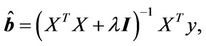 (5)
(5)
where λ is a positive constant, and  is the identity matrix. It can be seen from Equation (5) that adding λI to the matrix
  before inverting improves the conditioning of the estimation problem. The L2 regularization of the model parameters in RR makes it an effective means to achieve numerical stability in finding the solution and also to improve the predictive performance of the estimated inferential model.
3.2. Latent Variable Regression (LVR) Models
Dealing with the large number of highly correlated measured variables involved in inferential models is one of the key issues that affect their estimation and predictive abilities. It is known that over-parameterized models can fit the original data well, but they usually lead to poor predictions. Multivariate statistical projection methods such as PCR, PLS, and RCCA can be utilized to deal with this issue by performing regression on a smaller number of transformed variables, called latent variables (or principal components), which are linear combinations of the original variables. This approach, which is called latent variable regression (LVR), generally results in well-conditioned parameter estimates and good model predictions [9]. In the subsequent section, the problem formulations and solution techniques for PCR, PLS, and RCCA are presented.
However, before we introduce these methods, let’s introduce some definitions. Let the matrix D be defined as the augmented scaled input and output data, i.e., . Note that scaling the data is performed by making each variable (input and output) zero mean with a unit variance. Then, the covariance of D can be defined as follows [16]:
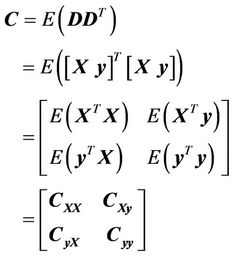 (6)
(6)
where the matrices ,
,  ,
,  and
and  are of dimensions
 ,
,  ,
,  , and
, and , respectively.
Since the latent variable model will be developed using transformed variables, let’s define the transformed inputs as follows:
 (7)
(7)
where  is the
  latent input variable
 , and
, and  is the
  input loading vector, which is of dimension
 .
.
3.2.1. Principal Component Regression (PCR)
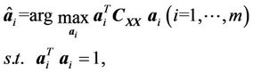
PCR accounts for collinearity in the input variables by reducing their dimension using principal component analysis (PCA), which utilizes singular value decomposition (SVD) to compute the latent variables or principal components. Then, it constructs a simple linear model between the latent variables and the output using ordinary least square (OLS) regression [5,10]. Therefore, PCR can be formulated as two consecutive estimation problems. First, the loading vectors are estimated by maximizing the variance of the estimated principal components as follows:
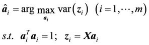 (8)
(8)
which, since the data are mean centered, can also be expressed in terms of the input covariance matrix  as follows:
 (9)
(9)
The solution of the optimization problem (9) can be obtained using the method of Lagrangian multiplier, which results in the following eigenvalue problem (see proof in Appendix A):
 (10)
(10)
which means that the estimated loading vectors are the eigenvectors of the matrix .
.
Secondly, after the principal components (PCs) are estimated, a subset (or all) of these PCs (which correspond to the largest eigenvalues) are used to construct a simple linear model, that relates these PCs to the output, using OLS. Let the subset of PCs used to construct the model be defined as , where
 , then the model relating these PCs to the output can be estimated as follows:
 (11)
(11)
which has the following solution,
 (12)
(12)
Note that if all the estimated principal components are used in constructing the inferential model (i.e., ), then PCR reduces to OLS. Note also that all principal components in PCR are estimated at the same time (using Equation (10)) and without taking the model output into account. Other methods that consider the input-output relationship into consideration when estimating the principal components include partial least squares (PLS) and regularized canonical correlation analysis (RCCA), which are presented next.
3.2.2. Partial Least Square (PLS)
PLS computes the input loading vectors,  , by maximizing the covariance between the estimated latent variable
  and model output,
  , i.e., [20,21]:
 (13)
(13)
where, . Since
  and the data are mean centered, equation (13) can also be expressed in terms of the covariance matrix
  as follows:
 (14)
(14)
The solution of the optimization problem 14 can be obtained using the method of Lagrangian multiplier, which leads to the following eigenvalue problem (see proof in Appendix B):
 (15)
(15)
which means that the estimated loading vectors are the eigenvectors of the matrix .
.
Note that PLS utilizes an iterative algorithm [20,22] to estimate the latent variables used in the model, where one latent variable or principal component is added iteratively to the model. After the inclusion of a latent variable, the input and output residuals are computed and the process is repeated using the residual data until a cross validation error criterion is minimized [5,10,22,23].
3.2.3. Regularized Canonical Correlation Analysis (RCCA)
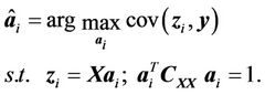
RCCA is an extension of a method called canonical correlation analysis (CCA), which was first proposed in [13]. CCA reduces the dimension of the model input space by exploiting the correlation among the input and output variables. The assumption behind CCA is that the input and output data contain some joint information that can be represented by the correlation between these variables. Thus, CCA computes the model loading vectors by maximizing the correlation between the estimated principal components and the model output [13-16], i.e.,
 (16)
(16)
where, . Since the correlation between two variables is the covariance divided by the product of the variances of the individual variables, Equation (16) can be written in terms of the covariance between
  and
and  subject to the following two additional constraints:
  and
and . Thus, the CCA formulation can be expressed as follows,
 (17)
(17)
Note that the constraint  is omitted from Equation (17) because it is satisfied by scaling the data to have a zero mean and a unit variance as described in Section 3.2. Since the data are mean centered, Equation (17) can be written in terms of the covariance matrix
  as follows:
 (18)
(18)
The solution of the optimization problem (18) can be obtained using the method of Lagrangian multiplier, which leads to the following eigenvalue problem (see proof in Appendix C):
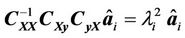 (19)
(19)
which means that the estimated loading vector is the eigenvector of the matrix .
.
Equation (19) shows that CCA requires inverting the matrix  to obtain the loading vector,
 . In the case of collinearity in the model input space, the matrix
  becomes nearly singular, which results in poor estimation of the loading vectors, and thus a poor model. Therefore, a regularized version of CCA (called RCCA) has been developed in [20] to account for this drawback of CCA. The formulation of RCCA can be expressed as follows:
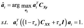 (20)
(20)
The solution of Equation (20) can be obtained using the method of Lagrangian multiplier, which leads to the following eigenvalue problem (see proof in Appendix D):
 (21)
(21)
which means that the estimated loading vectors are the eigenvectors of the matrix
 .
.
Note from Equation (21) that RCCA deals with possible collinearity in the model input space by inverting a weighted sum of the matrix  and the identity matrix, i.e.,
 instead of inverting the matrix
  itself. However, this requires knowledge of the weighting or regularizetion parameter
 . We know, however, that when
 , the RCCA solution (Equation (21)) reduces to the CCA solution (Equation (19)). On the other hand, when
 , the RCCA solution (Equation (21)) reduces to the PLS solution (Equation (15)) since
  is a scalar.
3.2.4. Optimizing the RCCA Regularization Parameter
The above discussion shows that depending on the value of , where
 , RCCA provides a solution that converges to CCA or PLS at the two end points, 0 or 1, respectively. The authors in [20] showed that RCCA can provide better results than PLS for some intermediate values of
  between 0 and 1. This observation motivated us to enhance the prediction ability of RCCA even further by optimizing its regularization parameter. To do that, in this section, we propose the following nested optimization problem to solve for the optimum value of
 :
:
 (22)
(22)
The inner loop of the optimization problem shown in Equation (22) solves for the RCCA model prediction given the value of the regularization parameter , and the outer loop selects the value of
  that provides the least cross validation mean square error using unseen testing data. The advantages of optimizing the regularization parameter in RCCA will be demonstrated through simulated examples in Section 4.
Note that RCCA solves for the latent variable regression model in an iterative fashion similar to PLS, where one latent variables is estimated in each iteration [20]. Then, the contributions of the latent variable and its corresponding model prediction are subtracted from the input and output data, and the process is repeated using the residual data until an optimum number of principal components or latent variables are used according to some cross validation error criterion. More details about the selection of optimum number of principal components are provided through the illustrative examples in the next section, which will provide some insight about the relative performances of the various inferential modeling methods and some of the practical issues associated with implementing these methods.
4. Illustrative Examples
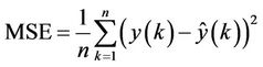
In this section, the performances of the inferential modeling techniques described in Section 3 and the advantages of optimizing the regularization parameters in RCCA are illustrated through two simulated examples. In the first example, models relating ten inputs and one output of synthetic data are estimated and compared using the various model estimation techniques. In the second example, on the other hand, inferential models predicting distillation column composition are estimated from measurements of other variables, such as temperature, flow rates, and reflux. In both examples, the estimated models are optimized and compared using cross validation, by minimizing the output prediction mean square error (MSE) using unseen testing data as follow,
 (23)
(23)
where  and
and  are the measured and predicted outputs at time step
 , and n is the total number testing measurements. Also, the number of retained latent variables (or principal components) by the various LVR modeling techniques (PCR, PLS, and RCCA) is optimized using cross validation. Finally, the data (inputs and output) are scaled (by subtracting the mean and dividing by the standard deviation) before constructing the models to enhance their prediction abilities. More details about the advantages of data scaling are presented in Section 4.1.3.
4.1. Example 1: Inferential Modeling of Synthetic Data
In this example, the performances of the various inferential modeling techniques are compared by modeling synthetic data consisting of ten input variables and one output.
4.1.1. Data Generation
The data are generated as follows. The first two input variables are “block” and “heavy-sine” signals, and the other input variables are computed as linear combinations of the first two inputs as follows:
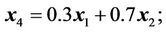
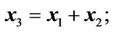
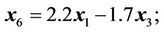
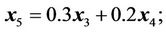
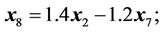
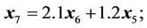
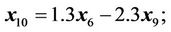
which means that the input matrix X is of rank 2. Then, the output is computed as a weighed sum of all inputs as follows:
 (24)
(24)
where,
for . The total number of generated data samples is 128. All variables, inputs and output, are assumed to be noise-free, which are then contaminated with additive zero mean Gaussian noise. Different levels of noise, which correspond to signal-to-noise ratios (SNR) of 10, 20, and 50, are used to illustrate the performances of the various methods at various noise contributions. The SNR is defined as the variance of the noise-free data divided by the variance of the contaminating noise. A sample of the output data, where SNR = 20 is shown in Figure 1.
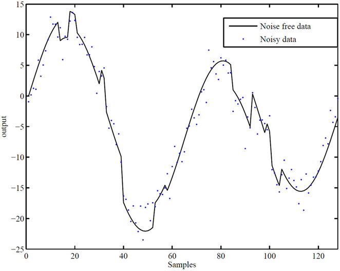
Figure 1. A sample output data set used in the synthetic example for the case where SNR = 20 (solid line: noise-free data; dots: noisy data).
4.1.2. Simulation Results
The simulated data are split into two sets: training and testing. The training data are used to estimate inferential models using the various modeling methods, and the testing data are used to compute the model prediction MSE (as shown in Equation (24)) using unseen data. To make statistically valid conclusions about the performances of the various modeling techniques, a Monte Carlo simulation of 1000 realizations is performed and the results are shown in Table 1 and Figure 2. These results show that the performance of RR is better than that of OLS, and that the performances of the LVR modeling techniques (PCR, PLS, and RCCA) clearly outperform the performances of the full rank models (OLS and RR). This is, in part, due to the fact that in LVR modeling, a portion of the noise in the input variables is removed with the neglected principal components, which enhances the model prediction. This is not the case in full rank models (OLS and RR) where all inputs are used to predict the model output. The results also show that the performances of PCR and PLS are comparable. These results agree with those reported in the literature [24,25], where the number of principal components is freely optimized for each model using cross validation and the models predictions are compared using unseen testing data. The optimum numbers of principal components used by the various LVR models for the case where  are shown in Figures 3(a), (c) and (e), which show that the optimum number of principal components used in PCR is usually more than what is used in PLS and RCCA to achieve a comparable prediction accuracy. The results in Table 1 and Figure 2 also show that RCCA provides a slight advantage over PCR and PLS when the optimum value of the regularization parameter
  is used. The value of
  is optimized using cross validation as shown in the RCCA problem formulation given in Equation (22). The optimization of
  for one realization is shown in Figure 4, in which
  is optimized by minimizing the cross validation MSE of the estimated RCCA model with respect to the testing data. Note also from Figures 3(a), (c) and (e), which compare the number of principal components used by the various
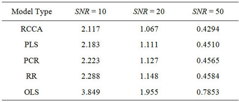
Table 1. Comparison between the prediction MSE’s obtained by the various modeling methods with respect to the noise-free testing data.
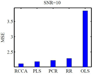
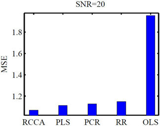
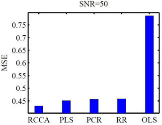
Figure 2. Histograms comparing the prediction MSE’s for the various modeling techniques and at different signal-tonoise ratios.
modeling methods, that RCCA is capable of providing this improvement using a smaller number of principal components than PCR and PLS.
4.1.3. Effect of Scaling the Data on the Predictions and Dimensions of Estimated Models
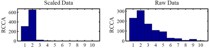
As mentioned earlier, scaled input and output data are used in this example to estimate the various inferential models. To illustrate the advantages of scaling the data (over using the raw data), the prediction and the number of principal components used (in the case of LVR models) are compared for the various model estimation techniques. To do that, a Monte Carlo simulation of 1000 realizations is performed to conduct this comparison, and the results are shown in Figures 3 and 5. Figure 5, which compares the MSE for the various modeling techniques using scaled and raw data, shows a clear advantage for data scaling on the models’ predictive abilities.
 (a)
(a)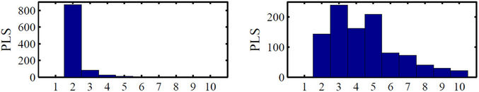 (b)
(b)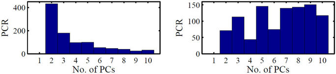 (c)
(c)
Figure 3. Histograms comparing the optimum number of principal components used by the various modeling techniques for scaled and raw data for the case where SNR = 20.
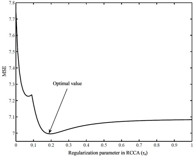
Figure 4. Optimization of the RCCA regularization parameter using cross validation with respect to the testing data.
Figure 3, on the other hand, which compares the effect of scaling on the optimum number of principal components (for PCR, PLS, and RCCA), shows that when scaled data are used, smaller numbers of PCs are needed for all model estimation techniques, and that RCCA uses the least number of PCs among all techniques.
4.2. Example 2: Inferential Modeling of Distillation Column Compositions
In this example, the various modeling techniques are compared when they are used to model the distillate and bottom stream compositions of a distillation column from other easily measured variables.
4.2.1. Process Description
The column used in this example, which is simulated using Aspen Plus, consists of 32 theoretical stages (including the reboiler and a total condenser). The feed stream, which is a binary mixture of propane and isobutene, enters the column at stage 16 as a saturated liquid. The feed stream has a flow rate of 1 kmol/s, a temperature of 322 K, and a propane composition of 0.4. The nominal steady state operating conditions of the column are presented in the Table 2.
4.2.2. Data Generation
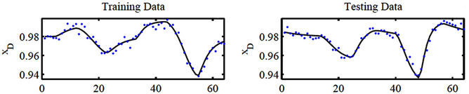
The data used in this modeling problem are generated by perturbing the flow rates of the feed and the reflux streams from their nominal operating conditions. First, step changes of magnitudes ±2% in the feed flow rate around its nominal condition are introduced, and in each case, the process is allowed to settle to a new steady state. After attaining the nominal conditions again, similar step changes of ±2% in the reflux flow rate around its nominal condition are introduced. These perturbations are used to generate training and testing data (each consisting of 64 data points) to be used in developing the various models. These perturbations (for the training and testing data sets) are shown in Figures 6(e)-(h).
In this simulated modeling problem, the input variables consist of ten temperatures at different trays of the column, in addition to the flow rates of the feed and reflux streams. The output variables, on the other hand, are the compositions of the light component (propane) in the
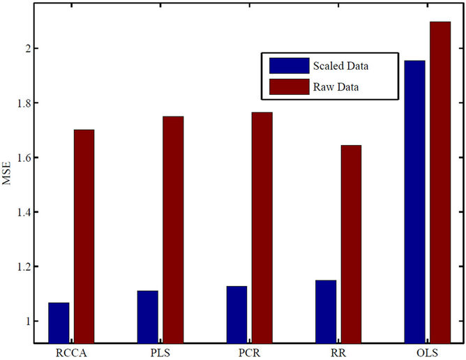
Figure 5. Comparison between the prediction MSE’s of the various modeling techniques using scaled and raw data for the case where SNR = 20.
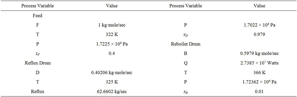
Table 2. Steady state operating conditions of the distillation column.
 (a)
(a)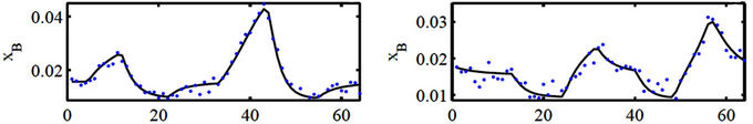 (b)
(b)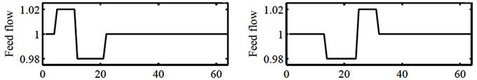 (c)
(c)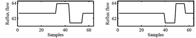 (d)
(d)
Figure 6. Sample data sets showing the changes in the feed and reflux flow rates and the resulting dynamic changes in the distillate and bottom stream compositions; For the composition data—solid line: noise-free data, dots: noisy data, SNR = 20.
distillate and bottom streams (i.e.,  and
and , respectively). The dynamic temperature and composition data generated using the Aspen simulator (due to the perturbations in the feed and reflux flow rates) are assumed to be noise-free, which are then contaminated with zeros mean Gaussian noise. To assess the robustness of the various modeling techniques to different noise contributions, different levels of noise (which correspond to signal-to-noise ratios of 10, 20 and 50) are used. Sample training and testing data sets showing the effect of the perturbations on the column compositions are shown in Figures 6(a)-(d) for the case where the signal-to-noise ratio is 20.
4.2.3. Simulation Results
The simulated distillation column data (training data and testing) used in this example are scaled as discussed in Example 1. The training data set are used to estimate the model, while the testing data are used to optimize and validate the quality of the estimated models. As performed in example 1, the number of principal components (in the case of LVR techniques, i.e., PCR, PLS, and RCCA) and other parameters (such as the regularization parameters, i.e., λ in RR or  in RCAA) are determined by minimizing the cross validation MSE for the unseen testing data.
To obtain statistically valid conclusions about the performances of the various modeling techniques, a Monte Carlo simulation of 1000 realizations is performed, and the results are presented in Figure 7 and Table 3. These results show that, in general, the LVR modeling methods (PCR, PLS, and RCCA) outperform the full rank methods (OLS and RR). The results also show that the performances of PCR and PLS are comparable, and that by optimizing its regularization parameter , RCCA can provide an improvement over these techniques. The value of
  is optimized using cross validation as shown in the RCCA problem formulation given in Equation (22). The optimization of
  for one realization for the output
  is shown in Figure 8. Finally, the results show that the prediction abilities of all modeling techniques degrade for larger noise contents, i.e., for smaller signal-to-noise ratios. The results obtained in this distillation column example agree with the results obtained in Example 1.
5. Conclusion
Inferential models are very commonly used in practice to estimate variables which are difficult to measure from other easier-to-measure variables. This paper presents a theoretical review, an extension to optimize RCCA for
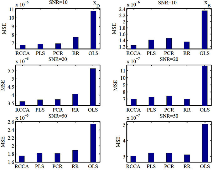
Figure 7. Histograms chart comparing the prediction MSE’s of the various modeling techniques using the distillation column data.
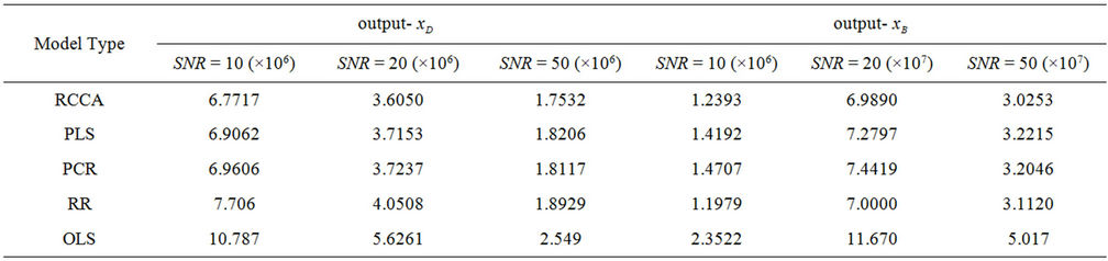
Table 3. Comparison between the prediction MSE’s (with respect to the noise-free testing data) of the distillate and bottom stream compositions for the various modeling techniques and at different signal-to-noise ratios.
enhanced prediction, as well as a comparative analysis for various inferential modeling techniques, which include ordinary least square (OLS) regression, ridge regression (RR), principal component regression (PCR), partial least square (PLS), and regularized canonical correlation analysis (RCCA). The theoretical review shows that the loading vectors used in LVR modeling can be computed by solving eigenvalue problems. For RCCA, it is shown that it can be optimized (to provide enhanced prediction ability) by optimizing its regularization parameter, which can be performed by solving a nested optimization problem. The various inferential modeling techniques are compared through two examples, one using synthetic data and the other using simulated distillation column data, where the distillate and bottom stream compositions are estimated using other easily measured variables. Both examples show that the latent variable regression (LVR) techniques (i.e., PCR, PLS, and RCCA) outperform the full rank techniques (i.e., OLS and RR). This is due to their ability to improve the conditioning of the model by neglecting principal components with small eigenvalues, and thus reducing the effect of noise on the model prediction. The obtained results also show that the performances of PCR and PLS are comparable when the number of principal components used are freely optimized using cross validation. Finally, it is shown that by optimizing its regularization parameter, RCCA can provide an improvement (in terms of its prediction MSE) over PCR and PLS using a smaller number of principal components.
6. Acknowledgements
This work was made possible by NPRP grant NPRP
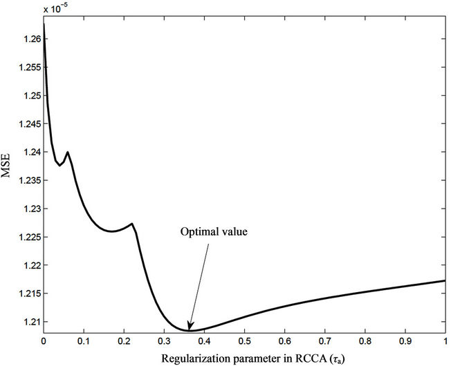
Figure 8. Optimization of the RCCA regularization parameter using cross validation with respect to the testing data.
09-530-2-199 from the Qatar National Research Fund (a member of Qatar Foundation). The statements made herein are solely the responsibility of the authors.
REFERENCES
- J. V. Kresta, T. E. Marlin and J. F. McGregor, “Development of Inferential Process Models Using PLS,” Computers & Chemical Engineering, Vol. 18, No. 7, 1994, pp. 597-611. doi:10.1016/0098-1354(93)E0006-U
- R. Weber and C. B. Brosilow, “The Use of Secondary Measurement to Improve Control,” AIChE Journal, Vol. 18, No. 3, 1972, pp. 614-623. doi:10.1002/aic.690180323
- B. Joseph and C. B. Brosilow, “Inferential Control Processes,” AIChE Journal, Vol. 24, No. 3, 1978, pp. 485-509. doi:10.1002/aic.690240313
- M. Morari and G. Stephanopoulos, “Optimal Selection of Secondary Measurements within the Framework of State Estimationin the Presence of Persistent Unknown Disturbances,” AIChE Journal, Vol. 26, No. 2, 1980, pp. 247- 259. doi:10.1002/aic.690260207
- I. Frank and J. Friedman, “A Statistical View of Some Chemometric Regression Tools,” Technometrics, Vol. 35, No. 2, 1993, pp. 109-148. doi:10.1080/00401706.1993.10485033
- A. Hoerl and R. Kennard, “Ridge Regression Based Estimation for Nonorthogonal Problems,” Technometrics, Vol. 8, 1970, pp. 27-52.
- J. McGregor, T. Kourti and J. Kresta, “Multivariate Identification: A Study of Several Methods,” IFAC ADCHEM Proceedings, Toulouse, Vol. 4, 1991, pp. 145-156.
- M. N. Nounou, “Dealing with Collinearity in Fir Models Using Bayesian Shrinkage,” Industrial and Engineering Chemistry Research, Vol. 45, 2006, pp. 292-298. doi:10.1021/ie048897m
- B. R. Kowalski and M. B. Seasholtz, “Recent Developments in Multivariate Calibration,” Journal of Chemometrics, Vol. 5, 1991, pp. 129-145. doi:10.1002/cem.1180050303
- M. Stone and R. J. Brooks, “Continuum Regression: Cross-Validated Sequentially Constructed Prediction Embracing Ordinaryleast Squares, Partial Least Squares and Principal Components Regression,” Journal of the Royal Statistical Society B, Vol. 52, No. 2, 1990, pp. 237-269.
- S. Wold, “Soft Modeling: The Basic Design and Some Extensions, Systems under Indirect Observations,” Elsevier, Amsterdam, 1982.
- E. Malthouse, A. Tamhane and R. Mah, “Non-Linear Partial Least Squares,” Computers and Chemical Engineering, Vol. 21, 1997, pp. 875-890. doi:10.1016/S0098-1354(96)00311-0
- H. Hotelling, “Relations between Two Sets of Variables,” Biometrika, Vol. 28, 1936, pp. 321-377.
- F. R. Bach and M. I. Jordan, “Kernel Independent Component Analysis,” Journal of Machine Learning Research, Vol. 3, No. 1, 2002, pp. 1-48.
- S. S. D. R. Hardoon and J. Shawetaylor, “Canonical Correlation Analysis: An Overview with Application to Learning Methods,” Neural Computation, Vol. 16, No. 12, 2004, pp. 2639-2664. doi:10.1162/0899766042321814
- M. Borga, T. Landelius and H. Knutsson, “A Unified Approach to PCA, PLS, MLR and CCA, Technical Report,” Technical Report, Linkoping University, 1997.
- T. Mejdell and S. Skogestad, “Estimation of Distillation Compositions from Multiple Temperature Measurements Using Partial Least Squares Regression,” Industrial & Engineering Chemistry Research, Vol. 30, 1991, pp. 2543-2555. doi:10.1021/ie00060a007
- M. kano, K. Miyazaki, S. Hasebe and I. Hashimoto, “Inferential Control System of distillation Compositions Using Dynamicpartial Least Squares Regression,” Journal of Process Control, Vol. 10, No. 2, 2000, pp. 157-166. doi:10.1016/S0959-1524(99)00027-X
- T. Mejdell and S. Skogestad, “Composition Estimator in a Pilot-Plant Distillation Column,” Industrial & Engineering Chemistry Research, Vol. 30, 1991, pp. 2555-2564. doi:10.1021/ie00060a008
- Y. Hiroyuki, Y. B. Hideki, F. C. E. O. Hiromu and F. Hideki, “Canonical Correlation Analysis for Multivariate Regression and Its Application to Metabolic Fingerprinting,” Biochemical Engineering Journal, Vol. 40, No. 2, 2008, pp. 199-204.
- R. Rosipal and N. Kramer, “Overview and Recent Advances in Partial Least Squares. Subspace, Latent Structure and Feature Selection Techniques,” Lecture Notes in Computer Science, Vol. 3940, 2006, pp. 34-51. doi:10.1007/11752790_2
- P. Geladi and B. R. Kowalski, “Partial Least Square Regression: A Tutorial,” Analytica Chimica Acta, Vol. 185, No. 1, 1986, pp. 1-17. doi:10.1016/0003-2670(86)80028-9
- S. Wold, “Cross-Validatory Estimation of the Number of Components in Factor and Principal Components Models,” Technometrics, Vol. 20, No. 4, 1978, p. 397. doi:10.1080/00401706.1978.10489693
- O. Yeniay and A. Goktas, “A Comparison of Partial Least Squares Regression with Other Prediction Methods,” Hacettepe Journal of Mathematics and Statistics, Vol. 31, 2002, pp. 99-111.
- P. D. Wentzell and L. V. Montoto, “Comparison of Principal Components Regression and Partial Least Square Regression through Generic Simulations of Complex Mixtures,” Chemometrics and Intelligent Laboratory Systems, Vol. 65, 2003, pp. 257-279. doi:10.1016/S0169-7439(02)00138-7
Appendix A. Determining the Loading Vectors Using PCR
Starting with the optimization problem shown in Equation (9), i.e.,
 (A.1)
(A.1)
the Lagrangian function for this optimization problem can be written as:
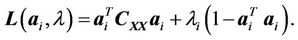 (A.2)
(A.2)
Taking the partial derivative of  with respect to
  and equating it to
 , we get,
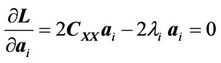 (A.3)
(A.3)
which gives the following eigenvalue problem:
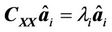 (A.4)
(A.4)
i.e., the loading vectors used in PCR are the eigenvectors of the covariance matrix .
.
Appendix B. Determining the Loading Vectors Using PLS
Starting with the optimization problem shown in Equation (14), i.e.,
 (B.1)
(B.1)
the Lagrangian function can be written as follows:
 (B.2)
(B.2)
Taking the partial derivative of  with respect to
  and equating it to
  we get,
 (B.3)
(B.3)
which gives the following eigenvalue problem,
 (B.4)
(B.4)
where, . Multiplying Equation (B.4) by
  and enforcing the constraint (
 ), we get,
 (B.5)
(B.5)
Taking the transpose of Equation (B.5), we get,
 (B.6)
(B.6)
Combing Equations (B.4) and (B.6), we get the following eigenvalue problem:
 (B.7)
(B.7)
Appendix C. Determining the Loading Vectors Using CCA
Starting with the optimization problem shown in Equation (18), i.e.,
 (C.1)
(C.1)
the Lagrangian function can be written as:
 (C.2)
(C.2)
Taking the partial derivative of  with respect to
  and equating it to
  we get,
 (C.3)
(C.3)
which gives the following solution,
 (C.4)
(C.4)
where  Multiplying Equation (C.4) by
  and enforcing the constraint (i.e.,
 ), we get,
 (C.5)
(C.5)
Taking the transpose of Equation (C.5), we get,
 (C.6)
(C.6)
Combing Equations (C.4) and (C.6), we get the following eigenvalue problem:
 (C.7)
(C.7)
Appendix D. Determining the Loading Vectors Using RCCA
Starting with the optimization problem shown in Equation (20), i.e.,
 (D.1)
(D.1)
the Lagrangian multiplier function can be written as follows:
 (D.2)
(D.2)
Taking the partial derivative of  with respect to
  and equating it to
 , we get,
 (D.3)
(D.3)
which gives the following solution:
 (D.4)
(D.4)
where . Multiplying Equation (D.4) by
and enforcing the constraint
(i.e., ), we get:
 (D.5)
(D.5)
Taking the transpose of Equation (D.5), we get,
 (D.6)
(D.6)
Combining Equations (D.4) and (D.6), we get the following eigenvalue problem:
 (D.7)
(D.7)
NOTES
*Corresponding author.