Materials Sciences and Applications
Vol.4 No.1(2013), Article ID:27083,26 pages DOI:10.4236/msa.2013.41010
FE Modeling and Analysis of Isotropic and Orthotropic Beams Using First Order Shear Deformation Theory
![]()
Aeronautical Department, Military Technical Collage, Cairo, Egypt.
Email: *maelshafei@yahoo.com
Received October 26th, 2012; revised November 12th, 2012; accepted December 11th, 2012
Keywords: Finite Element Method; Timoshenko Beam Theory; Composite Materials Mechanics; Static and Dynamic Analysis of Beams
ABSTRACT
In the present work, a finite element model is developed to analyze the response of isotropic and orthotropic beams, a common structural element for aeronautics and astronautic applications. The assumed field displacements equations of the beams are represented by a first order shear deformation theory, the Timoshenko beam theory. The equations of motion of the beams are derived using Hamilton’s principle. The shear correction factor is used to improve the obtained results. A MATLAB code is constructed to compute the natural frequencies and the static deformations for both types of beams with different boundary conditions. Numerical calculations are carried out to clarify the effects of the thickness-to-length ratio on both the Eigen values and the deflections of the beams due to the applied mechanical load. The obtained results of the proposed model are compared to the available results of other investigators, good agreement is generally obtained.
1. Introduction
The current trend of aeronautics and astronautic design is to use large, complex, and light-weight structures elements. These structures are commonly having low-frequency fundamental vibration modes in addition to fabricate by graphite-epoxy to satisfy the requirements of minimum weight and low thermal distortion. Because of that several researchers are interested to solve the beam structures by different theories.
Yuan and Miller [1], proposed finite element model for laminated composite beams with separate rotational degrees of freedom for each lamina. The shear deformation is included in the model but the interfacial slip or delamination is not included. Their element can be used even for short beams with many laminas. The model results was compared with those of other theoretical and experimental investigations and found reasonable.
Chandrashekhara and Bangera [2], developed finite element model based on a higher-order deformation theory with Poisson’s effect is incorporated. They concluded the following: 1) The shear deformations decrease the natural frequencies of the beam; 2) The natural frequencies increase with the increase of the number of beam layers; 3) The clamped-free boundary condition exhibits the lowest frequencies; 4) The increase of fiber orientation angle decreases the natural frequency; and 5) the natural frequency decreases by increasing the material anisotropy.
Friedman and Kosmatka [3], developed two-node Timoshenko beam element using Hamilton’s principal. The resulting stiffness matrix of their model was exactly integrated and it was free of “shear-locking”, and it was in agreement with the exact Timoshenko beam stiffness matrix. Their element was exactly predicting the displacement of short beam subjected to distributed loads and also predicted the natural frequencies.
Lidstrom [4], derived an equilibrium formulation of 3D beam element using the energy derivatives. His formulation contains the coupling terms between translation and twist, also between translational bending and elongation. A three node element was introduced in such model. Also condensed two node version of the element has been analyzed. He found that two-node system was less numerically stable than the proposed three-node system.
Bhate et al. [5], proposed a refined flexural theory for composite beam based on the potential energy concept. The warping effect is included in their formulation; however the shear correction coefficient was eliminated. They found that their theory is established for short composite beams where cross-sectional warping is predominant.
Nabi and Ganesan [6], studied the free vibration characteristics of composite beams using finite element model based on a first-order deformation theory including bi-axial bending as well as torsion. They studied the effect of shear-deformation, beam geometry, and boundary conditions on the natural frequencies. They concluded that the natural frequencies are 1) Decrease with the increase of fiber orientation angle; 2) Increase with the increase of the beam length to height ratio for all fiber orientation angles; 3) Also have the lowest value in case of clamped-free boundary conditions Armanios and Badir [7], evaluated analytically the effect of elastic coupling mechanisms on vibration behaveior of thin-walled composite beams. Good agreement was found between their results and those developed by Giavotto et al. (1983) [8], and Hagodes et al. (1991) [9], based on finite element technique, and the experimental measurements obtained by Chandra and Chopra [10].
Rao and Ganesan [11], investigated a Harmonic response of tapered composite beams using finite element model based on a higher order shear deformation theory. The uniaxial bending and the Poisson ratio effect were considered and the interlaminar shear stresses were neglected. The effect of in-plane inertia and rotary inertia were also considered in their formulation of the mass matrix. A parametric study is done of the influence of anisotropy, taper profile and taper parameter. They found that the transversal displacement is higher than that of a uniform beam. For the taper parameter effect, they deduced that the frequency decreases with increase thickness variations and vise-verse.
Khdeir and Reddy [12], presented an exact solution of the governing equations for the bending of laminated beams. They used the classical, the first-order, the second-order, and the third-order beam theories in their analysis. They studied the effect of shear deformation, number of layers, and the orthotropic ratio on the static response of composite beams. They found large differences between the predicted deflections by the classical beam theory and the higher order beam theories, especially when the ratio of beam length to its height was low due to the shear deformation effects.
Yildirim et al. [13], studied the in-plane free vibration of laminated beams based on the transfer matrix method. They considered rotary inertia, shear, and extensional deformation effects on the Timoshenko’s beam analysis. Good predictions are obtained and compared to other reporters for different modes of the natural frequencies.
Chakraborty et al. [14], proposed a refined looking free first order shear deformable finite element model to solve free vibration and wave propagation problems in laminated composite beam. They developed element, that its shape functions is dependent not only on the length of the element, but also on its material and cross-sectional properties. The developed stiffness matrix is exact while the mass distribution is approximate. Rotary inertia and effect of geometric and material asymmetry is taken into account. They named the model as refined first order deformable element (RFSDE).
Eisenberger [15], proposed exact stiffness coefficients for isotropic beam using a simple higher order theory, which include cubic variation of the axial displacements over the cross-section of the beam. Their model had three degrees of freedom at each node, one transverse displacement and two rotations. They compared their model results with Bernoulli-Euler and Timoshenko beam models and found acceptable.
Lee and Schultz [16], studied the free vibration of Timoshenko beams and axi-symmetric Mindlin plates. The analysis was based on the Chebyshev pseudospectral method, which has been widely used in the solution of fluid mechanics problems. Different boundary conditions of Timoshenko beams were treated, and numerical results were presented for different thickness-to-length ratios.
Subramanian [17], proposed free vibration analysis of composite beams using Finite elements based on two higher order shear deformation theories. The difference between the two theories is that the first theory assumed a non-parabolic variation of transverse shear stress across the thickness of the beams whereas the second theory assumed parabolic variation. The comparison study showed that natural frequencies predict by his model were better than those obtained by other theories and the considered finite elements.
Simsek and Kocaturk [18], studied the free vibration of isotropic beams based on the third-order shear deformation theory. The boundary conditions are satisfied using Lagrange multipliers which reduced the solution of a system of algebraic equations. A trial functions for the deflections and rotations of the cross-section of the beam are expressed in polynomial form. Their results are compared with the previous results based on CBT and FSDT.
Jun et al. [19], proposed dynamic finite element model for beams based of first-order shear deformation theory. They introduced the influences of Poisson effect, couplings among extensional, bending and torsion deformations, shear deformation and rotary inertia in their formulation. Their obtained results are compared to those previously published and founded in good accuracy.
Lee and Janga [20], presented spectral element model for axially loaded bending-torsion coupled composite beam based on the first-order shear deformation theory, Timoshenko beam model. They found that the use of frequency-dependent spectral element matrix i.e. exact dynamic stiffness matrix, provide extremely accurate solutions, while reducing the total number of degreesof-freedom to resolve the computational and cost problems.
Nguyen et al. [21], presented full closed-form solution of the governing equations of two-layer composite beam. Timoshenko’s kinematics assumptions are considered for both layers and the shear connection is modeled through a continuous relationship between the interface shear flow and the corresponding slip. They derived the “exact” stiffness matrix using the direct stiffness method. They found that the effect of shear flexibility on the deflection is generally more important for composite beams characterized by substantial shear interaction.
Lina and Zhang [22], proposed a two-node element with only two degrees of freedom per node for finite element analyses of isotropic and composite beams. Their model was based on Timoshenko theory. They concluded that their proposed model is accurate and computationally efficient for analysis of isotropic and composite beams.
Kennedya et al. [23], presented Timoshenko beam theory for layered orthotropic beams. The proposed theory yields Cowper’s shear correction for single isotropic layer, while for multiple layers new expressions for the shear correction factor are obtained. The body-force correction was shown to account for the difference between Cowper’s shear correction and the factor originally proposed by Timoshenko. Numerical comparisons between the theory and finite-elements results showed good agreement.
In the present work, a finite element model is proposed, based on first order shear deformation theory, Timoshenko beam theory, with a shear correction factor, to predict the static responses and dynamic characteristics of advanced isotropic and orthotropic beams for different boundary conditions and different length to thickness ratio due to different applied loads. The structure outline of the present work can be drawn for both isotropic and orthotropic beams as follows:
1) Theoretical formulation using the Timoshenko theory.
2) Finite element formulation to obtain the structure equation of motion.
3) The model validation and parametric studies which contain the items:
a) Model convergence for both deflection and eigenvalues.
b) Static deformation of the beam.
c) Dynamic characteristics of the beam.
d) Model predictions analysis and conclusions.
2. Theoretical Formulation
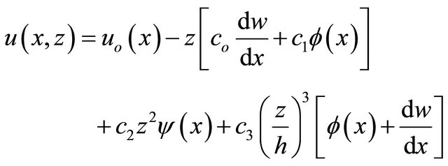
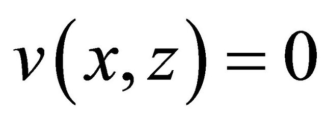
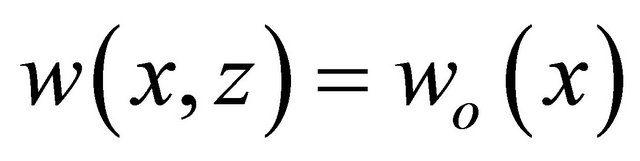
The displacements field equations of the beam are assumed as follows [12]:
 (1a)
(1a)
 (1b)
(1b)
 (1c)
(1c)
where ,
,  and
and  are the displacements field equations along the coordinates
 and
and , respectively,
  and
and  denote the displacements of a point
  at the mid plane,
 and
and  are the rotation angles of the cross-section as shown in Figure 1.
By selecting the constant values of Equation (1) a as:

 , the displacements field equations for first-order theory (FOBT) at any point through the thickness can be expressed as [24]:
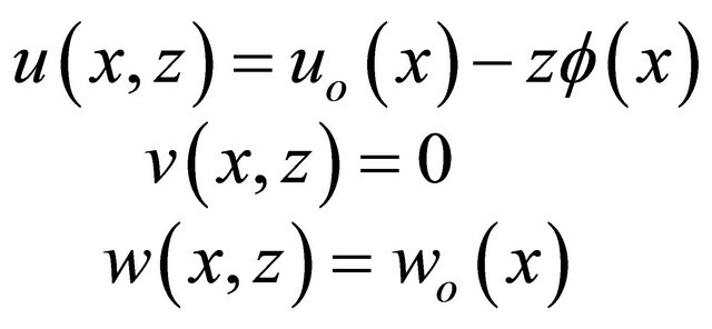 (2)
(2)
The strain-displacement relationships are obtained by differentiating the assumed displacement field equations, Equation (2), as follows:
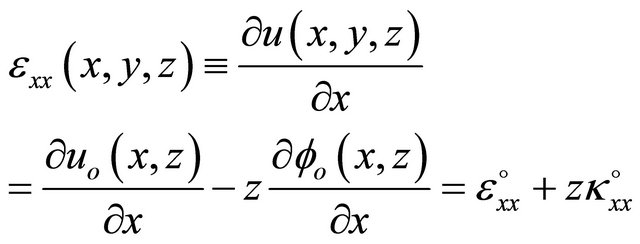 (3a)
(3a)
 (3b)
(3b)
The strains at any point through the thickness of the beam can be written in matrix form as:
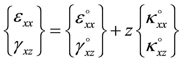 (4)
(4)
The components 
 and
and  are the reference surface extensional strain in the x-direction, in-plane shear strain, and curvature in the x-direction, respectively.
The generalize stress strain relationship is given by [25]:
 (5)
(5)
where, ; and
; and .
.
The plane stress approximations are made by setting the stress component in the transverse direction , and eliminate the corresponding strain
  from the constitutive relation, Equation (5) as follows [25]:
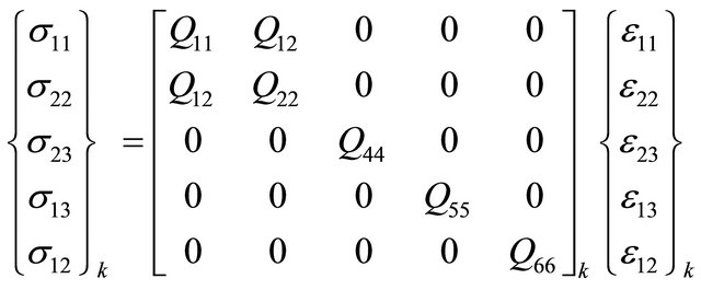 (6)
(6)
where,  are the reduced stiffness components which related to the engineering constants for two material cases such as:
Case I: Isotropic Beam
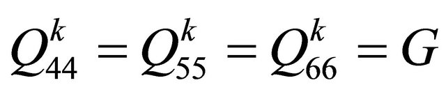
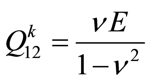
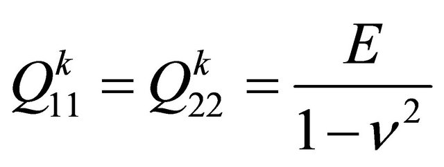 (7a)
(7a)
where;  , G, and
  are the material properties.
Case II: Orthotropic Beam
 (7b)
(7b)
where;  is the modules in
  direction,
  are the shear modules in the
  plane, and
  are the associated Poisson’s ratios.
Thus the transformed stress-strain relationship can be written as:
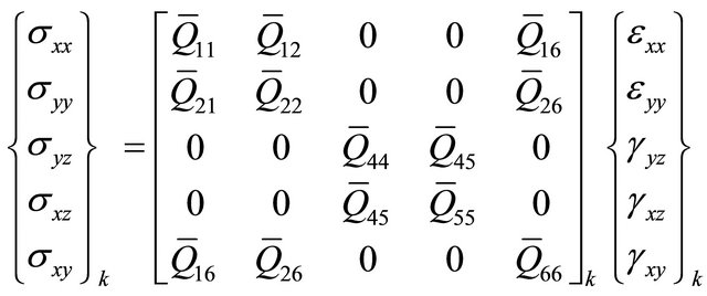 (8)
(8)
where,  , are the transformed reduced stiffness components [25].
In the present model the width in y direction is stress free and a plane stress assumptions are used. Therefore, it is possible to set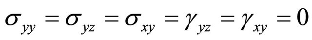 , and
, and 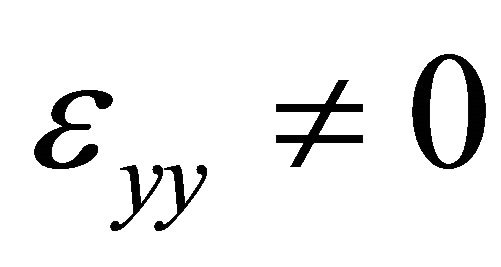 in Equation (8). Therefore, the stress-strain relationship can be reduced to:
 (9a)
(9a)
where;  is the shear correction factor and the coefficients in Equation (9a) are given by:
Case I: Isotropic beam
 (9b)
(9b)
Case II: Orthotropic Beam
 (9c)
(9c)
3. Energy Formulation
The kinetic energy of the beam structure is given by [6]:
 (10)
(10)
where, ρ is the mass density of the material of the beam.
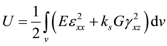
The internal strain energy  for the beam structure is represented by [12]:
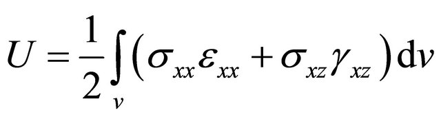 (11)
(11)
And the work done due to external loads is represented by [24]:
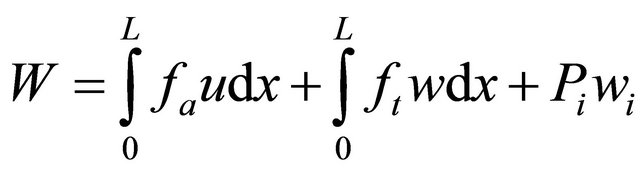 (12)
(12)
where;  and
and  are the transversal and axial forces along a surface with length
 , respectively.
 , is the concentrated force at point
  and
and  is the corresponding generalized displacement.
Case I: Isotropic beam
By substituting Equations (9a), and (9b) into Equation (11), the internal strain energy is represented by:
 (13)
(13)
By inserting Equations (3a), and (3b) into Equation (13), one can obtain:
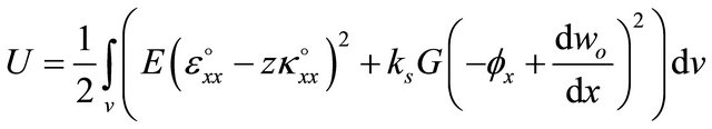 (14a)
(14a)
 (14b)
(14b)
Thus;
 (15)
(15)
Case II: Orthotropic Beam
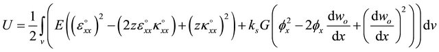
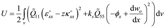
By substituting Equation (9a) in Equation (11), the internal strain energy of the composite beam is represented by:
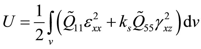 (16)
(16)
By inserting Equations (3a), and (3b) into Equation (16)one can obtain:
 (17a)
(17a)
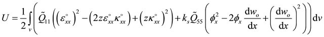 (17b)
(17b)
And performing the integration through the thickness, the internal strain energy for anisotropic beam is represented by:
 (18)
(18)
where,  and
and  are the laminate extensional, coupling, and bending stiffness coefficients and they are given by [25]:
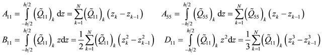 (19)
(19)
4. Finite Element Formulation
In the present model the proposed element has five nodes with nine degrees of freedom representing the deformations  and
and  as shown in the Figure 2.
A cubic shape functions are used to represent the axial displacement , quadratic shape functions for the transverse displacement
 , where the rotation
  is represented by a linear shape functions, this will result a nine by nine stiffness matrix with different degrees of freedom at different nodes [24]. From these selections we have:
 , and
, and 
Which satisfied the constrains, shear strain
 , and membrane strain
 , to avoid the error in the finite element analysis which is known as shear Locking due to un-accurately models the curvature present in the actual material under bending, and a shear stress is introduced. The additional shear stress in the element causes the element to reach equilibrium with smaller displacement, i.e., it makes the element appear to be stiffer than it actually is and gives bending displacements smaller than they should be. The axial displacement at the mid-plane
  is expressed as the following:
 (20)
(20)
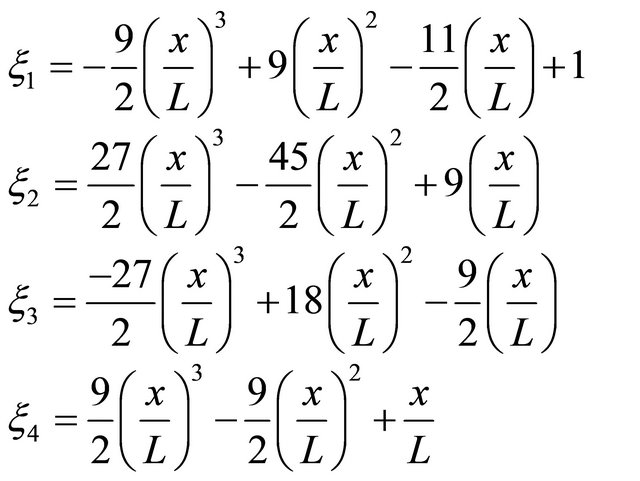
By solving the previous equation and imposing the boundary conditions, the axial displacement can be represented as:
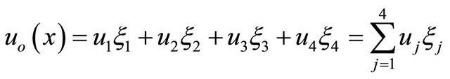 (21)
(21)
where the cubic shape functions  are found to be [26]:
 (22)
(22)
The transversal displacement  is represented as:
 (23)
(23)
By solving the above equation and applying the boundary conditions to determine the unknown constants, the transversal displacement  can be expressed in terms of the nodal displacement as:
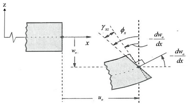
Figure 1. Deformed and un-deformed shape of Timoshenko beam [24].

Figure 2. Element nodal degrees of freedom.
 (24)
(24)
where, the quadratic interpolation shape functions are given by [26]:
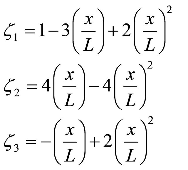 (25)
(25)
The rotation angle  is expressed as:
 (26)
(26)
Similarly; by solving Equation (26) and applying the boundary conditions, the rotation angle is given by:
 (27)
(27)
where the Linear interpolation shape functions  have the form [27]:
 , and
, and  (28)
(28)
5. Variational Formulation
The mathematical statement of Hamilton’s principle can be expressed as [3]:
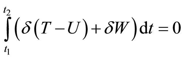 (29)
(29)
where,  denote the first variation,
  and
and  are two arbitrary time variables except that at
 , and
, and , all variation are zero. The advantage of this method is that it accounts for the physics of the entire structure simultaneously. Starting with the first integral and assume that each layer of the present composite beam model has the same vibration speed.
Thus the first variation of the kinetic energy Equation (10) is expressed as:
 (30)
(30)
By inserting Equation (2) into Equation (30) yields:
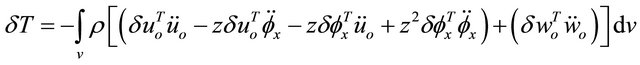 (31)
(31)
By substituting the shape functions Equations. (21), (24), and (27) in Equation (31) the components of the element mass matrix can be expressed by:
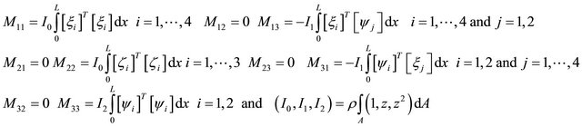 (32)
(32)
where,  is the mass moment of inertia.
By inserting Equations (22), (25), and (28) into Equation (32) and perform the integrating, the element mass matrix is obtained, and given in Appendix A.
The first variation of the external work Equation (12) takes the form:
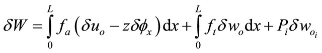 (33)
(33)
By inserting the shape functions Equations. (21), (24), and (27) into Equation (33), one can obtain:
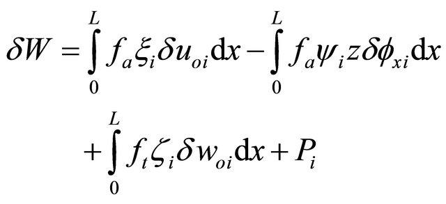 (34)
(34)
Thus, the elements of the load vector are as follows:
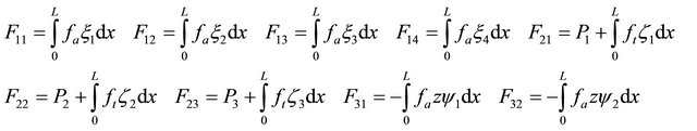 (35)
(35)
By substituting Equations (22), (25), and (28) in Equation (35) and perform the integrating, the element load vector can be obtained and given in Appendix A.
Case I: Isotropic beam:
By taking the variation of Equation (15), one can obtain:
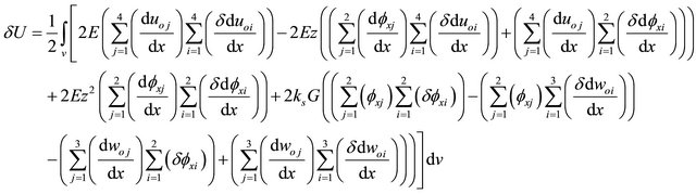 (36)
(36)
By substituting Equations (21), (24) and (27) in Equation (36) yields:
 (37)
(37)
Equation (37) defines the elements of the stiffness matrix as follows:
 (38)
(38)
By inserting Equation (22), (25) and (28) into Equation (38), and perform the integration, the element stiffness matrix for isotropic Timoshenko Beam is obtained and given in Appendix A.
Case II: Orthotropic Beam:
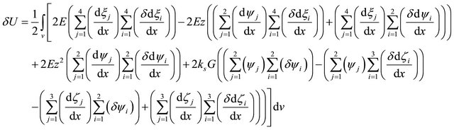
By taking the variation of Equation (18), one can obtain:
 (39)
(39)
By inserting Equations (21), (24) and (27) into Equation (39) yields the form given in Equation (40):
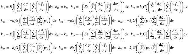
The element stiffness matrix can be deduced from Equation (40) as shown in Equation (41):
By substituting Equation (22), (25) and (28) in Equation (41) and perform the integration, the element stiffness matrix of anisotropic Timoshenko beam is obtained and given in Appendix A.
6. Equation of Motion
The system equation of motion is given in matrix form as [11]:
 (42)
(42)
where  is the global mass matrix,
  is the second derivative of the nodal displacements with respect to time,
  is the global stiffness matrix,
  is the nodal displacements vector and
  is the global nodal forces vector.
7. Numerical Example and Discussion
A MATLAB code is constructed to perform the analysis of isotropic and orthotropic beams using the present finite element model. The model is capable of predicting the nodal (axial and transversal) deflections and the fundamental natural frequency of the beam. The model inputs are the materials and geometric properties of the beams. The shear correction factor is taken as k = 5/6, and the following boundary conditions of the beams are considered as follows:
Simply-supported edge:  and
and .
.
Clamped edge: ,
,  , and
, and .
.
The model validation is performed by checking the convergences for deflection and eigen-values, static deflections and dynamic characteristics for both isotropic and orthotropic beams.
Case I: Isotropic beam results
1) Model Convergences
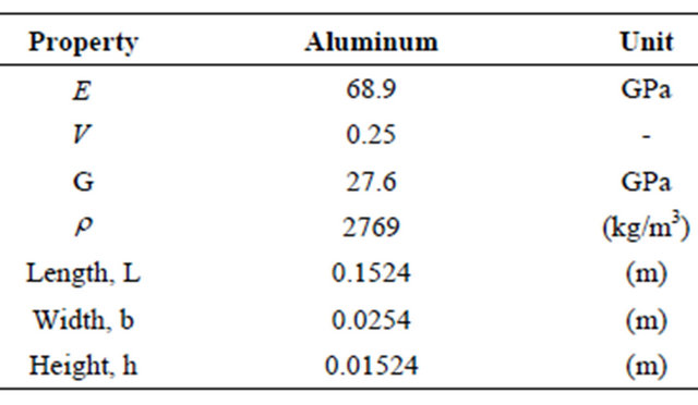
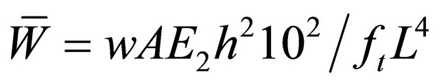
The convergence of the present model is checked for the aluminum beam with the material and geometric properties given in Table 1. The beam is subjected to uniform distributed load of intensity 1 N/m. The obtained results are shown in Figure 3, which presents the effect of number of element on the normalized transversal tip deflection of a cantilever beam, with length to height ratio (L/h) of 10, The normalized deflection is given as; . It can be seen from the figure that the model predictions are start to converge at reasonable number of elements.
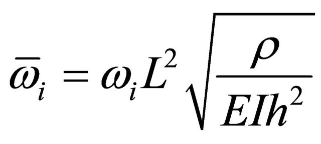
The convergence of the Eigen values is checked for two cases of the beam boundary conditions clamped-free and clamped-clamped where the dimensionless frequency
 is defined as:
 , and
, and  is the mass per unit length of the beam.
a) Clamped-free aluminum beam with the properties given in Table 1. The obtained dimensionless first natural frequency is conversing by increasing the number of elements as shown in Figure 4.
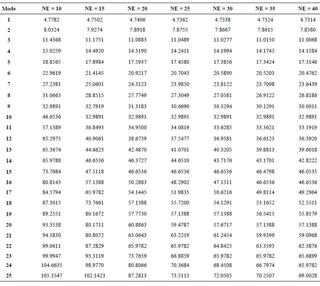
b) Clamped-Clamped aluminum beam with the properties: Poisson’s ratio  thickness to length ratio is h/L=0.01, and the number of elements are chosen from 10 to 40. The obtained normalized natural frequencies are presented in Table 2 for different number of ele-

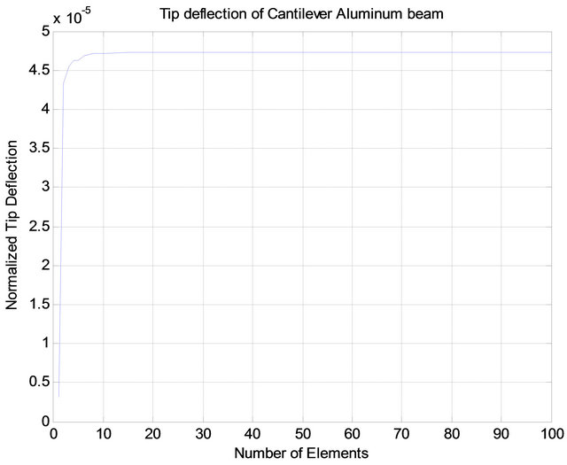
Figure 3. Normalized transversal tip displacements vs. number of elements of cantilever aluminum beam.
Table 1. Material and geometric properties for aluminum beam.
ments “NE”. The obtained results are found reasonable and compared with the predictions given by [16], which used different numbers of collocation points to determine the size of the problem in their studies It is clear from Figure 4 and Table 2 that as the number of elements increase the natural frequency decreases for the first and other modes.
2) Static Validation
Example (1):
A cantilever isotropic beam with cross-section dimensions ,
, , and
, and  are used in the validation in order to compared with other references. The beam is subjected to transverse uniform distributed loads with intensity
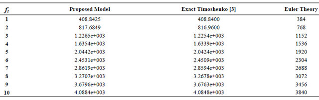
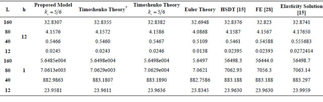
  up to 10 N/m, and with different values of length to thickness ratio L/h = 4, 10, 20, 50, and 100. In the present example, the shear correction factor is taken as
  and number of elements, NE = 33, are taken in the proposed model in order to compare the results to other references. The obtained results are presented and in Table 3(a)-(e) and compared to [3], where the Timoshenko–based tip deflection is given as:
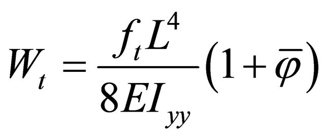 ,
, 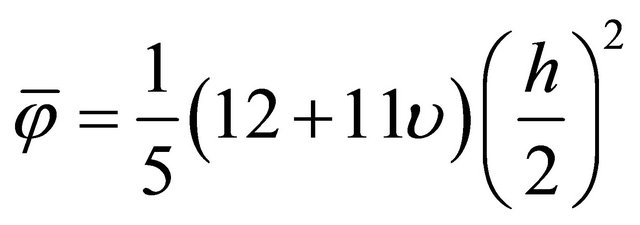 and its shear correction factor is
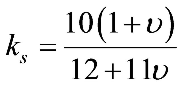 . Also compared with the known Euler formula for max tip deflection,
 .
.
It is shown from the previous tables that for L/h less than 20 the proposed model gives results more accurate then the exact formula of Timoshenko and Euler beams. For L/h greater than 20 the values of the obtained results are start to be less than Timoshenko based solution and gradually get closer to Euler solution.
Example (2):
A cantilever beam with the following properties: ,
, ,
,  subjected to tip load
  as given by [15]. It is shown from the obtained results given in Table 4 the following: 1) the model accuracy is in between the HSDT and the finite element and other different solutions; 2) also the effect of the shear correction factor on the obtained results.
3) Dynamic Validation
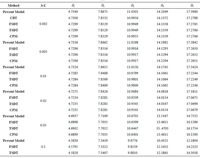
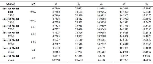
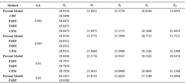
The free vibration validation is performed for the aluminum beam with material properties given in Table 1. The obtained results are given in Table 5. to Table 7. for beams with different boundary conditions with NE = 35 and the ratio h/L = 0.002 to 0.2. The obtained dimensionless frequencies  are compared with the previously published results of CBT [28], FSDT [29], TSDT [18], and CPM [16].
For clamped-clamped beam, Table 5(a) shows the following for the first five modes:
1) For h/L = 0.2, the present model results are better than TODT but less than FSDT, and CPM.
2) For h/L less than or equal 0.1, the present model is less than all other theories.
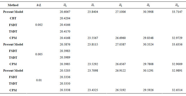
Table 5(b) shows the following for the next five modes (6 - 10):
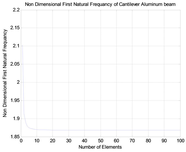
Figure 4. Non-dimensional first natural frequency vs. number of elements of cantilever aluminum beam.
Table 2. Convergence test of the non-dimensional frequency  of clamped-clamped aluminum beam with the number of elements.
1) For h/L equal to or grater than 0.1, the present model is gives more accurate results than all theories by significant values, and this difference increase by increasing the mode number.
2) For all modes as the ratio h/L increases the natural frequencies decreases.
Table 6(a) shows the first five modes of Free-Free beam it is clear that:
1) As long as h/L less than or equal to 0.05 the obtained results are closed to CBT and CBM theories.
2) For h/L greater than or equal to 0.05 the model results are better than other theories.
Table 6(b) shows the next five modes (6 - 10), for F-F beam as long as h/L less than 0.05 the proposed model gives less accuracy than CPM and CBT theories. For the ratio L/h less than or equal 0.05 the model results are better than CPM theory.
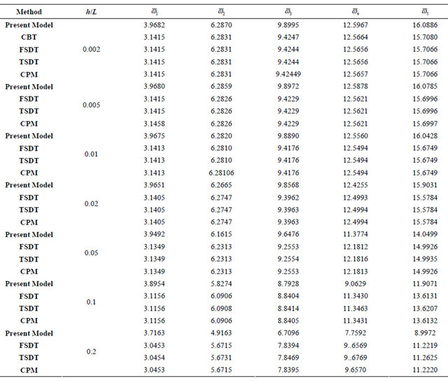
It seen from Table 7(a) for the first five modes of the S-S beam the proposed model gives results closer to all other theories for all values of h/L.
Table 7(b) shows the modes 6 to 10 for S-S beam it is clear that as long as h/L less than or equal to 0.02, the proposed model gives results closed to other theories. For the ratio h/L greater than or equal 0.05 the model results are better than all other theories with remarkable values.
CASE II: Orthotropic Beam Results
a) Model convergences
The convergence of the present model is checked for the orthotropic beam with the material properties given as;

 , and
, and . A cantilever composite beams with different orientation angles [45/-45/45/-45], [30/50/30/50], and [0/90/0/90] with length to height ratio (L/h) is equal to 10, are used. The beam is subjected to uniform distributed load
  of intensity 1 N/m. Figure 5 shows the effect of number of element on the normalized transversal
Table 3. (a) Transverse tip deflection of isotropic cantilever beam for different values of applied loads (L/h = 4); (b) Transverse tip deflection of isotropic cantilever beam for different values of applied loads (L/h = 10); (c) Transverse tip deflection of isotropic cantilever beam for different values of applied loads (L/h = 20); (d) Transverse tip deflection of isotropic cantilever beam for different values of applied loads (L/h = 50); (e) Transverse tip deflection of isotropic cantilever beam for different values of applied loads (L/h = 100).
(a)
(b)
(c)
(d)
(e)

Table 4. Transverse tip deflection of isotropic cantilever beam compared with other theories.
*Shear correction factor is: .
.
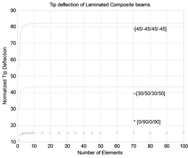
Figure 5. Normalized transverse tip deflections vs. number of elements of cantilever composite beams.
tip deflection of beams which is given as:
 , where
  is the actual transversal deflection. It can be seen that the model predicttions are start to converge at reasonable number of elements for the different beams with different orientation angles.
In case of free vibration, the convergences of the natural frequencies of orthotropic beams with the same properties given above in this section are checked for two cases. The dimensionless frequency  is defined as:
1) First case: Clamped-free beam with different orienttation angles [45/-45/45/-45], [30/50/30/50], and [0/90/ 0/90]. The obtained results of the dimensionless first natural frequency are shown in Figure 6 for different number of elements.
2) Second Case: Clamped-free and clamped-clamped composite beams with stacking sequences [45/-45/45/ -45], with number of elements changed from 10 to 40. The obtained results are presented in Tables 8 and 9.
It is clear from Figure 6, Tables 8 and 9 that as the number of elements increases the natural frequency decreases until it reaches a constant value.
b) Static Validation
To check the validity of the model for orthotropic beam, two layer [0/90], three layer [0/90/0], four layer [0/90/0/90] and 10-layer [0/90/0/90..] lay-up are considered with material properties given above (case II:
Table 5. (a) Non-dimensional frequency  of clamped-clamped aluminum beam (Modes: 1 - 5); (b) Non-dimensional frequency
 of clamped-clamped aluminum beam (Modes: 6 - 10).
(a)
(b)
Continued
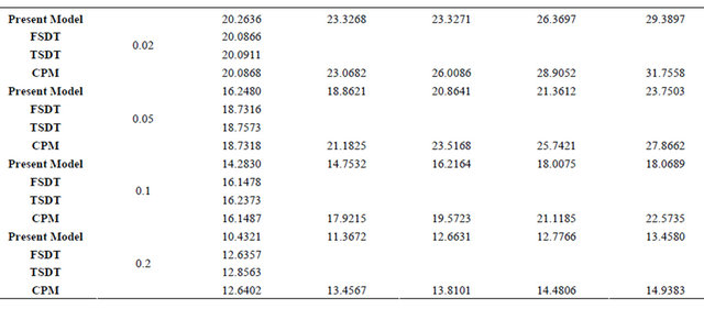
Table 6. (a) Non-dimensional frequency  of Free-Free aluminum beam (Modes: 1 - 5); (b) Non-dimensional frequency
  of Free-Free aluminum beam (Modes: 6 - 10).
(a)
(b)
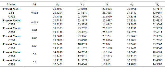
Table 7. (a) Non-dimensional frequency  of simply supported aluminum beam (Modes: 1 - 5); (b) Non-dimensional frequency
  of simply supported aluminum beam (Modes: 6 - 10).
(a)
(b)
Continued
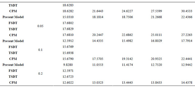
Table 8. Convergence Test of the Non-dimensional frequency  of clamped-free composite beam [45/-45/45/-45] for different number of elements.
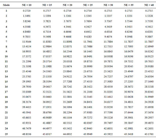
Table 9. Convergence Test of the Non-dimensional frequency  of clamped-clamped composite beam [45/-45/45/-45] for different number of elements.
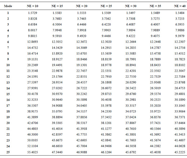
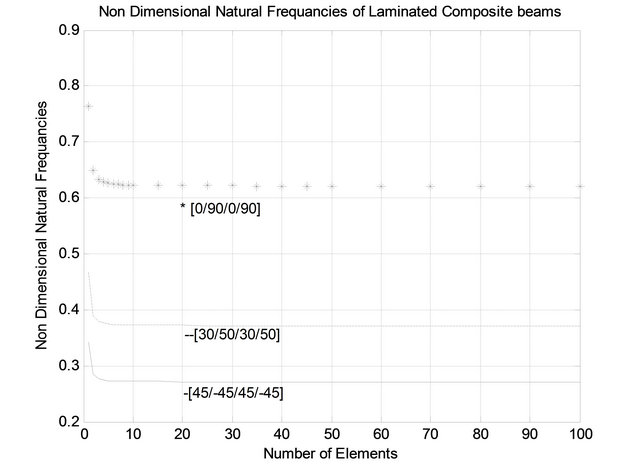
Figure 6. Non-dimensional first natural frequency vs. number of elements of cantilever composite beams.
orthotropic beam). Different length to height ratio L/h = 5, 10, and 50 are used to validate the proposed model. All laminas are assumed to be of the same thickness and made of the same materials. The number of elements is taken equal to 33. The mid span deflection is chosen in the validation in order to compare the obtained results with different theories reported in [12] and [14]. These predictions are given in Tables 10-12.
Table 10. (a) Non-dimensional mid-span deflection of symmetric cross-ply beams [0/90/0] for various boundary conditions; (b) Non-dimensional mid-span deflection of anti-symmetric cross-ply beams [0/90] for various boundary conditions.
(a)
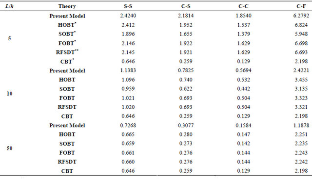
*Reference [12]. **Reference [14].
(b)
*Reference [12]. **Reference [14].
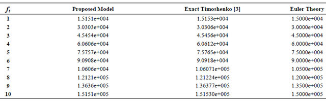
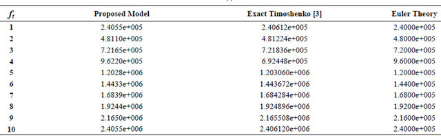
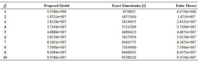
Table 11. Comparison of natural frequencies (kHz) of simply supported composite beams.
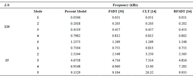
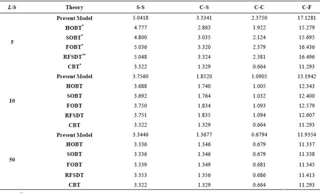
Table 12. Comparison of non-dimensional natural frequencies of symmetrically laminated cross-ply and angle-ply beams under various boundary conditions.

It is shown in Table 10(a) that the non-dimensional mid-span deflections of symmetric cross-ply beams are better than CBT, FSDT and HSDT theories for all L/h ratios, however for C-F case it is better than CBT only and poor than FSDT and HSDT theories, known that the a few seconds are taken to complete the single run of the code.
It is shown in Table 10(b) that the non-dimensional mid-span deflections of symmetric cross-ply beams are better than all theories for all values of L/h ratios, for the various proposed boundary conditions. Large differences between the results of the refined theories and the classical theory are noted, especially when the L/h ratio decreases (L/h less than or equal to 5), indicating the effect of shear deformation. It is seen that the symmetric cross-ply stacking sequence gives a smaller response than those of anti symmetric ones. The obtained results by the present model are close to the predictions of FOBT theory and the RFSDT reported in [12] and [14].
c) Dynamic Validation
To check the free vibration validity of the present model, An AS/3501-6 graphite/epoxy composite used in the analysis with the following properties:
 ,
,  ,
,  ,
,
 ,
,  , and
, and
 . The beam length to height ratio is
 . The non-dimensional fundamental natural frequency is given by:
 , where
  and
and
 are the free natural frequency and mass of the material of the beam, respectively. All laminas are assumed to be of the same thickness and made of the same materials. The obtained results are given in Tables 11-13, and they compared with different theories reported in [2], [14], and [30].
Table 11 shows the comparisons of the first five natural frequencies of a long thin (L/h = 120) and a short thick (L/h = 15) simply supported unidirectional  composite beam. It seen that the proposed element prediction are better than the results obtained from the RFSDT [14], which used the same assumed displacement equations as the present model, but its element has two nodes with total six degrees of freedom. Also the present model predictions are in good agreement with the available results for both thin and thick beams.
Table 12 shows the comparison of the non-dimensional natural frequencies of symmetrically laminated cross-ply [0/90/0/90] and angle-ply [45/-45/45/-45] beams for various boundaries. For cross-ply the obtained results are much closed to the results obtained by other methods (exact FSDT, RFSDT, and HSDT). For angle-ply the obtained results are much closer to the results of [6] using HSDT with FE, and deviate from the results of the exact solution [30] which reported in [2], and the results obtained from RFSDT [14].
Table 13 shows the first five natural frequencies for different un-symmetrically lamination in comparison with [2], good agreement is found.
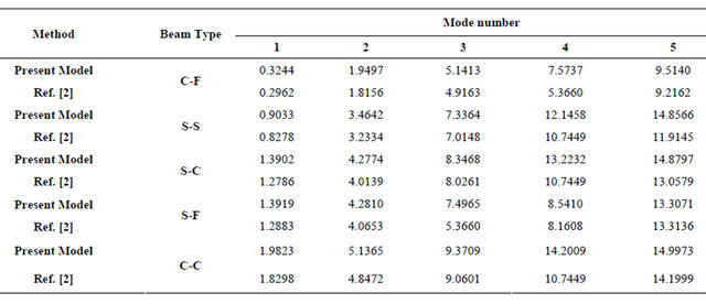
The effect of the boundary conditions on the first five natural frequencies of anti-symmetric angle ply beams is shown in Table 14. The obtained results from the present model for different boundary conditions are much closed to the results of [2], which used HSDT.
8. Conclusions
The following conclusions have been drawn:
1) Finite element model has been obtained for static deformation and free vibration analysis of isotropic and orthotropic beams based on first order shear deformation theory, Timoshenko beam theory.
2) Various results have been presented to show the effect of number of elements, boundary conditions, length to thickness ratio L/h, material properties, number of layers, and ply orientation, on the static deflection and natural frequency of the proposed models.
3) The proposed model is valid to decrease the error due to un-accurately modeling of the curvature present in the actual material under bending which known as shear Locking.
4) The code running time is around few second for both deflection and natural frequency calculation using number of elements equal 33 on PC Pentium 3.
5) The model results are converging at small number of elements for deflection and natural frequency for isotropic and orthotropic beams.
6) In case isotropic beam subjected to uniform distributed loads the static analysis shows that for length to thickness ratio L/h less than 20 the proposed model gives more accurate results than the exact formula of Timoshenko and Euler beams. For L/h greater than 20 the obtained results values are start to be less than Timoshenko based solution and get gradually closer to Euler solution.
7) Also for isotropic beam subjected to concentrated tip load the model accuracy is in between the HSDT, the finite element and other different solutions. Also the shear correction factor affects the obtained results.
Table 13. Effect of ply orientation angles on the non-dimensional natural frequencies of un-symmetric clamped-clamped beams.
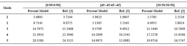
Table 14. Effect of boundary conditions on the non-dimensional natural frequencies of anti-symmetric laminated angle ply beams [45/-45/45/-45].
8) In case isotropic beam, generally, for small value of L/h (h/L equal to or greater than 0.05), the model results are better than all other theories CBT, exact FSDT (EFSDT), CPT, and HSDT for various boundary conditions. However, for the ratio L/h greater than a value around 20, generally, the model results were closer to the results of other theories.
9) For cross-ply orthotropic composite beams the obtained deflections are better than all other theories for all values of L/h and for all boundary conditions, except (C-F) case, the EFSDT and HSDT were better. However, for angle-ply beams the proposed model is better than all.
10) For cross-ply and angle-ply orthotropic composite beam the natural frequency are accepted in compared with EFSDT and HSDT, and better than RFSDT.
11) The model gives natural frequency of composite beam better than EFSDT and HSDT for S-S, S-F, C-C boundary conditions, and it were closer to these theories for other C-F and S-S boundary conditions.
REFERENCES
- F. G. Yuan and R. E. Miller, “A New Finite Element for Laminated Composite Beams,” Computers and Structures, Vol. 31, No. 5, 1989, pp. 737-745. doi:10.1016/0045-7949(89)90207-1
- K. Chandrashekhara and K. M. Bangera, “Free Vibration of Composite Beams Using a Refined Shear Flexible Beam Element,” Computers and Structures, Vol. 43, No. 4, 1992, pp. 719-727. doi:10.1016/0045-7949(92)90514-Z
- Z. Friedman and J. B. Kosmatka, “An Improved TwoNode Timoshenko Beam Finite Element,” Computer and Structures, Vol. 47, No. 3, 1993, pp. 473-481. doi:10.1016/0045-7949(93)90243-7
- T. Lidstrom, “An Analytical Energy Expression for Equilibrium Analysis of 3-D Timoshenko Beam Element,” Computers and Structures, Vol. 52, No. 1, 1994, pp. 95- 101. doi:10.1016/0045-7949(94)90259-3
- S. R. Bhate, U. N. Nayak and A. V. Patki, “Deformation of Composite Beam Using Refined Theory,” Computers and Structures, Vol. 54, No. 3, 1995, pp. 541-546. doi:10.1016/0045-7949(94)00354-6
- S. M. Nabi and N. Ganesan, “Generalized Element for the Free Vibration Analysis of Composite Beams,” Computers and Structures, Vol. 51, No. 5, 1994, pp. 607-610. doi:10.1016/0045-7949(94)90068-X
- E. A. Armanios and A. M. Badir, “Free Vibration Analysis of the Anisotropic Thin-Walled Closed-Section Beams,” Journal of the American Institute of Aeronautics and Astronautics, Vol. 33, No. 10, 1995, pp. 1905-1910. doi:10.2514/3.12744
- V. Giavotto, M. Borri, P. Mantegazza, G. Ghiringhelli, V. Carmash, G. Maffioli and F. Mussi, “Anisotropic Beam Theory And Applications,” Computers and Structures, Vol. 16, No. 4, 1983, pp. 403-413. doi:10.1016/0045-7949(83)90179-7
- D. Hagodes, A. Atilgan, M. Fulton and L. Rehfield, “Free Vibration Analysis of Composite Beams,” Journal of the American Helicopter Society, Vol. 36, No. 3, 1991, pp. 36-47. doi:10.4050/JAHS.36.36
- R. Chandra and I. Chopra, “Experimental and Theoretical Investigation of the Vibration Characteristics of Rotating Composite Box Beams,” Journal of Aircraft, Vol. 29, No. 4, 1992, pp. 657-664. doi:10.2514/3.46216
- S. R. Rao and N. Ganesan, “Dynamic Response of Tapered Composites Beams Using Higher Order Shear Deformation Theory,” Journal of Sound and Vibration, Vol. 187, No. 5, 1995, pp. 737-756. doi:10.1006/jsvi.1995.0560
- A. A. Khdeir and J. N. Reddy, “An Exact Solution for the Bending of Thin and Thick Cross-Ply Laminated Beams,” Computers and Structures, Vol. 37, 1997, pp. 195-203. doi:10.1016/S0263-8223(97)80012-8
- V. Yildirm, E. Sancaktar and E. Kiral, “Comparison of the In-Plan Natural Frequencies of Symmetric Cross-Ply Laminated Beams Based On The Bernoulli-Eurler and Timoshenko Beam Theories,” Journal of Applied Mechanics, Vol. 66, No. 2, 1999, pp. 410-417. doi:10.1115/1.2791064
- A. Chakraborty, D. R. Mahapatra and S. Gopalakrishnan, “Finite Element Analysis of Free vibration and Wave Propagation in Asymmetric Composite Beams With Structural Discontinuities,” Composite Structures, Vol. 55, No. 1, 2002, pp. 23-36. doi:10.1016/S0263-8223(01)00130-1
- M. Eisenberger, “An Exact High Order Beam Element,” Computer and Structures, Vol. 81, No. 3, 2003, pp. 147- 152. doi:10.1016/S0045-7949(02)00438-8
- J. Lee and W. W. Schultz, “Eigenvalue Analysis of Timoshenko Beams and Axi-symmetric Mindlin Plates by the Pseudospectral Method,” Journal of Sound and Vibration, Vol. 269, No. 3-5, 2004, pp. 609-621. doi:10.1016/S0022-460X(03)00047-6
- P. Subramanian, “Dynamic Analysis of Laminated Composite Beams Using Higher Order Theories and Finite Elements,” Composite and Structures, Vol. 73, No. 3, 2006, pp. 342-353. doi:10.1016/j.compstruct.2005.02.002
- M. Simsek and T. Kocaturk, “Free Vibration Analyses of Beams by Using a Third-Order Shear Deformation Theory,” Sadana, Vol. 32, Part 3, 2007, pp. 167-179. doi:10.1007/s12046-007-0015-9
- L. Jun, H. Hongxinga and S. Rongyinga, “Dynamic Finite Element Method for Generally Laminated Composite Beams,” International Journal of Mechanical Sciences, Vol. 50, No. 3, 2008, pp. 466-480. doi:10.1016/j.ijmecsci.2007.09.014
- U. Lee and I. Jang, “Spectral Element Model for Axially Loaded Bending-Shear-Torsion Coupled Composite Timoshenko Beams,” Composite Structures, Vol. 92, No. 12, 2010, pp. 2860-2870. doi:10.1016/j.compstruct.2010.04.012
- Q. H. Nguyen, E. Martinellib and M. Hjiaja, “Derivation of the Exact Stiffness Matrix for a Two-Layer Timoshenko Beam Element with Partial Interaction,” Engineering Structures, Vol. 33, No. 2, 2011, pp. 298-307. doi:10.1016/j.engstruct.2010.10.006
- X. Lina and Y. X. Zhang, “A Novel One-Dimensional Two-Node Shear-Flexible Layered Composite Beam Element,” Finite Elements in Analysis and Design, Vol. 47, No. 7, 2011, pp. 676-682. doi:10.1016/j.finel.2011.01.010
- G. J. Kennedya, J. S. Hansena and J. R. R. A Martinsb, “A Timoshenko Beam Theory with Pressure Corrections for Layered Orthotropic Beams,” International Journal of Solids and Structures, Vol. 48, No. 16-17, 2011, pp. 2373- 2382. doi:10.1016/j.ijsolstr.2011.04.009
- J. N. Reddy, “An Introduction to Nonlinear Finite Element Analysis,” Oxford University Press, USA, 2004.
- J. N. Reddy, “Mechanics of Laminated Composite Plates and Shells-Theory and Analysis,” 2nd Edition, CRC Press, USA, 2004.
- S. S. Rao, “The Finite Element Method in Engineering,” 2nd Edition, BPCC Wheatons Ltd., Exeter, 1989, pp. 206-207.
- R. D. Cook, D. S. Malkus and M. E. Plesha, “Concept and Applications of Finite Element Analysis,” 3rd Edition, John Wiley & Sons, 1974, p. 96.
- W. C. Hurty and M. F. Rubinstein, “Dynamics of Structures,” Prentice Hall, New Delhi, 1967.
- T. Kocaturk and M. Simsek, “Free Vibration Analysis of Timoshenko Beams under Various Boundary Conditions,” Sigma Journal of Engineering and Natural Science, Vol. 1, 2005, pp. 30-44.
- K. Chandrashekhara, K. Krishnamurthy and S. Roy, “Free Vibration of Composite Beams Using a Refined Shear Flexible Beam Element,” Computers and Structures, Vol. 14, No. 4, 1990, pp. 269-279. doi:10.1016/0263-8223(90)90010-C
Appendix A
The element mass matrix for the Timoshenko Beam:
 (A-1)
(A-1)
where; 
The element stiffness matrix for orthotropic Timoshenko Beam:
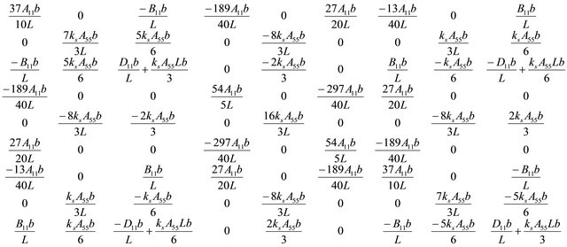 (A-2)
(A-2)
The element load vector:
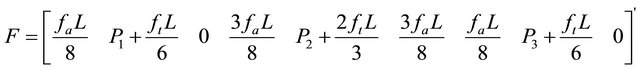 (A-3)
(A-3)
The element stiffness matrix for isotropic Timoshenko Beam is:
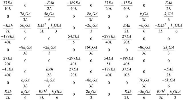 (A-4)
(A-4)
where; 
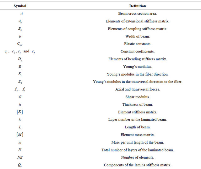
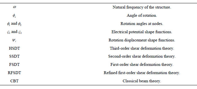
Nomenclature

NOTES
*Corresponding author.