Journal of Modern Physics
Vol.4 No.6(2013), Article ID:32998,8 pages DOI:10.4236/jmp.2013.46106
Localisation Inverse Problem and Dirichlet-to-Neumann Operator for Absorbing Laplacian Transport
École centrale Paris, Laboratoire de MSS-MAT, F-92295 Grande voie des Vignes, Châtenay-Malabry cedex, France
Email: ibrahim.baydoun@ecp.fr
Copyright © 2013 Ibrahim Baydoun. This is an open access article distributed under the Creative Commons Attribution License, which permits unrestricted use, distribution, and reproduction in any medium, provided the original work is properly cited.
Received March 18, 2013; revised April 18, 2013; accepted May 13, 2013
Keywords: Absorbing Laplacian Transport; Dirichlet-to-Neumann Operators; Inverse Problem
ABSTRACT
We study Laplacian transport by the Dirichlet-to-Neumann formalism in isotropic media . Our main results concern the solution of the localisation inverse problem of absorbing domains and its relative Dirichlet-to-Neumann operator
 . In this paper, we define explicitly operator
 , and we show that Green-Ostrogradski theorem is adopted to this type of problem in three dimensional case.
1. Laplacian Transport and Dirichlet-to-Neumann Operators
The theory of Dirichlet-to-Neumann operators is the basis of many research domains in analysis, particularly, those concerning Laplacian transports. It is also very important in mathematical-physics, geophysics, electrochemistry. Moreover, it is very useful in medical diagnosis, such as electrical impedance tomography:
In 1989, J. Lee and G. Uhlmann have introduced an example on the determination of conductivity matrix field in a bounded open domain, see e.g. [1]. This example is related to measuring the elliptic Dirichlet-toNeumann map for associated conductivity equation, see e.g. [1].
The problem of electrical current flux is an example of so-called diffusive Laplacian transport. Besides the voltage-to-current problem, the motivation to study this kind of transport comes for instance, from the transfer across biological membranes, see e.g. [2,3].
Let some species of concentration ,
,  , diffuse stationary in the isotropic bulk
  from a (distant) source localised on the closed boundary
  towards a semipermeable compact interface
  of the cell
 , where they disappear at a given rate
 . Then the steady field of concentrations (Laplacian transport with a diffusion coefficient
 ) obeys the set of equations:
(P1) 
Usually, one supposes that ,
,  , is a constant concentration of the species inside the cell
 .
.
This example motivates the following abstract stationary diffusive Laplacian transport problem with absorption on the surface :
:
(P2) 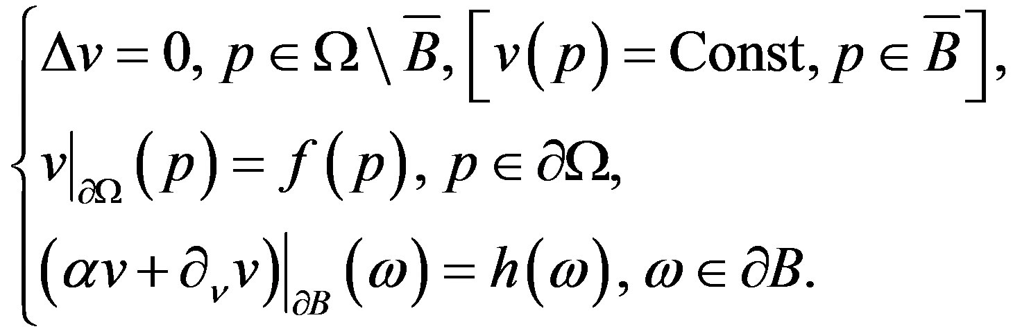
This is the Dirichlet-Neumann problem for domain  with the Robin [4] boundary condition on the absorbing surface
 . Varying
  between
  and
and , one recovers respectively the Neumann and the Dirichlet boundary conditions.
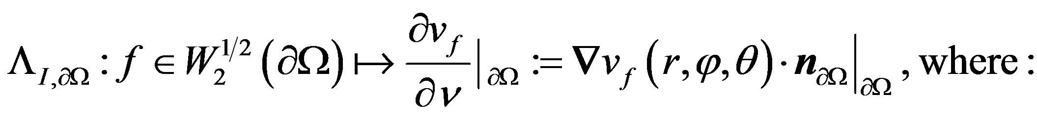
Now, we can associate with the problem (P2) a Dirihlet-to-Neumann operator
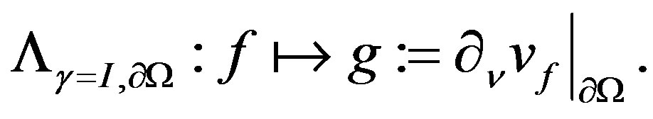 (1)
(1)
Domain  belongs to a certain Sobolev space of functions on the boundary
 , which contains
 , the solutions of the problem (P2) for given
 and for the Robin boundary condition on
  fixed by
  and
and .
.
The advantage of this approach is that as soon as the operator (1) is defined, one can apply it to study the mixed boundary value problem (P2). This gives, in particularly, the value of the particle flux due to Laplacian transport across the membrane . Moreover, the total current across the boundary
  can be defined (for given
 ) in term of Dirihlet-to-Neumann operator (1) as follows:
 (2)
(2)
where  designed the differential element relative to
 .
.
There are at least two inverse problems derived from problem (P2):
a) geometrical inverse problem: given Dirichlet data  and the corresponding (measured) Neumann data
 , in (1), on the accessible outer boundary
 , to reconstruct the shape of the interior boundary
 , see [5].
b) localisation inverse problem: concerns to localisate of the domain (cell)  with a given shape and the fixed parameters
  and
and , see [6].
The main question in this context is to find sufficient conditions insuring that the localization inverse problem is uniquely soluble. Indeed:
First, we relate the above problems a) and b) with the Dirichlet-to-Neumann operator (1) by defining explicitly this operator, whose can define the local and total current across the external boundary , which are useful to resolve a) and b).
Second, we study the localisation inverse problem in the framework of application outlined in the problem (P2), which consist in finding sufficient (Dirichlet-toNeumann) conditions to localise the position of the cell  from the experimentally measurable macroscopic response parameters.
In Section 2, we introduce the existence and uniqueness for the solution of problem (P2). In Section 3, we introduce our first main result concerning the study of spherical case of problem (P1), whose we give a general method to resolve the type of partial derivative system like (P1), see proposition 3.2. Indeed, we allow an explicit calculations, based on Green-Ostrogradski theorem, for the solution of this problem.
In Section 4, it is our second main result which consist in showing that total current across the external boundary , involving Dirihlet-to-Neumann operator (1), can resolve the localisation inverse problem in three dimensional case, when the compact
 .
.
2. Uniqueness of the Problem (P2)
We suppose that  and
and  be open bounded domains in
  with
with  -smooth disjoint boundaries
  and
and , that is
  and
and  .
.
Then the unit outer-normal to the boundary  vector-field
  is well-defined, and we consider the normal derivative in (P2) as the interior limit:
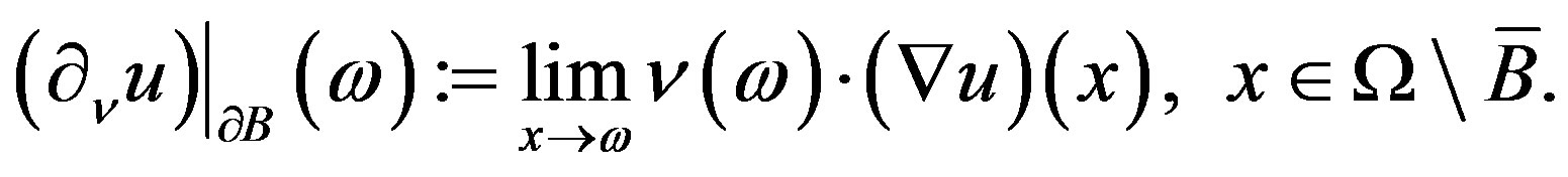 (3)
(3)
The existence of the limit (3) as well as the restriction 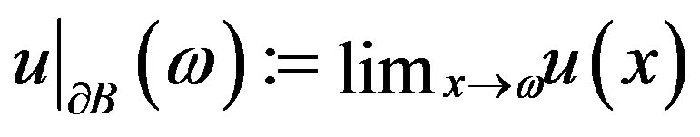 is insured since
  has to be harmonic solution of problem (P2) for
  -smooth boundaries
  [7].
[7].
Now, we introduce some indispensable standard notations and definitions, see [8]. Let  be Hilbert space
  on domain
  and
and  denote the corresponding boundary space. We denote by
  the Sobolev space of
  -functions, whose
  derivatives are also in
 , and similar,
  is the Sobolev space of
  -functions on the
  -smooth boundary
 .
.
Proposition 2.1. Let  for
for  -smooth boundaries
 . Then the Dirichlet-Neumann problem (P2) has a unique (harmonic) solution in domain
 .
.
Proof. For existence we refer to [7]. To prove the uniqueness, we consider the problem (P2) for  and
and . Then by Gauss-Ostrogradsky theorem, one gets that the corresponding solution
  yields:
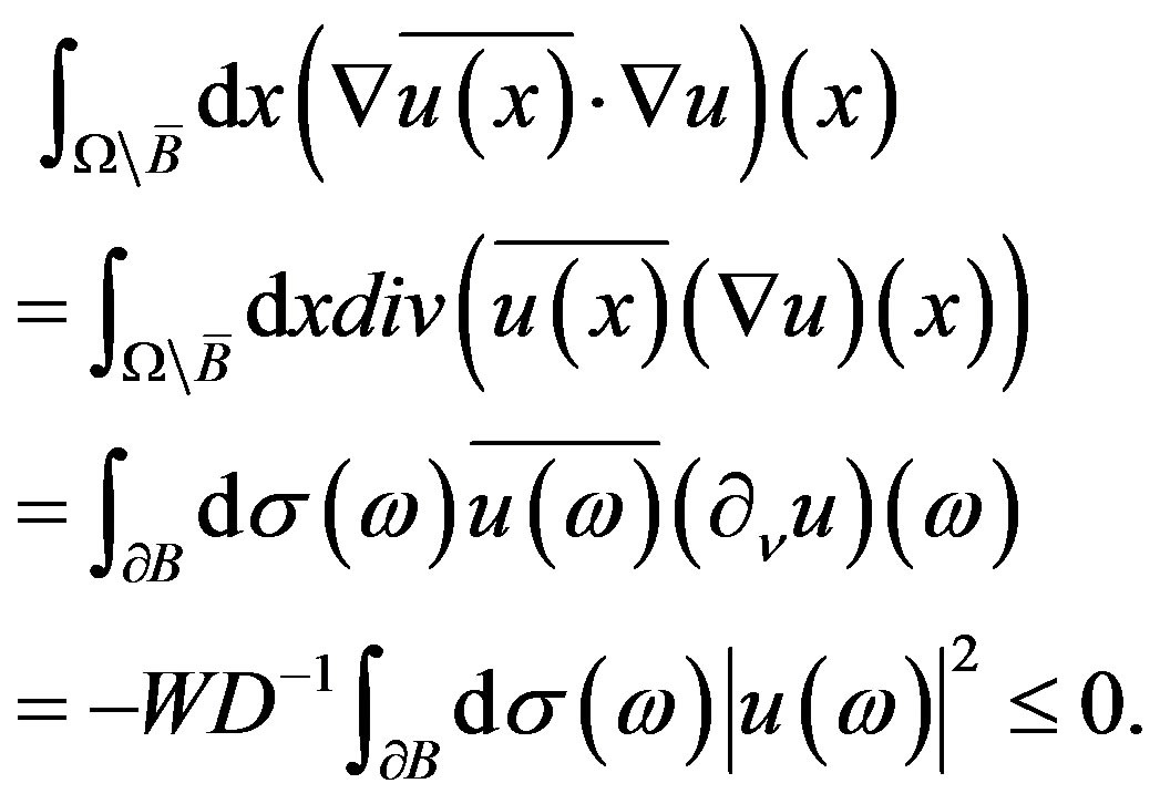 (4)
(4)
The estimate (4) implies that . Hence by the boundary condition one gets
 , and from
 we obtain that for
 , the harmonic function
  for
for .
. 
The next statement is a key for analysis of inverse localisation problems:
Proposition 2.2. Consider two problems (P2) corresponding to a bounded domain  with
with  - smooth boundary
  and to two subsets
  and
and  with the same smoothness of the boundaries
 ,
, . If for solutions
 ,
,  of these problems one has
 (5)
(5)
then .
.
Proof. By virtue of  and by condition (5), the problem (P2) has two solutions for identical external (on
 ) and internal (on
  and
and ) Robin boundary conditions. Then by the standard arguments based on the Holmgren uniqueness theorem [9] for harmonic functions on
 , one obtains that
 .
. 
3. Dirichlet-to-Neumann Operators for Absorbing Laplacian Transport
Here, we consider the spherical shell of the problem (P1) so that  and the absorbing cell is also a ball
 , whose we denote by
  the distance between the two centers
 .
.
Hereafter, we denote the previous hypothesis by spherical case.
In the sequel, we resolve the problem (P1) in order to calculate explicitly Dirichlet-to-Neumann operator relative to this case.
Before resolving problem (P1), we need the following theorem which the key of the solution:
Theorem 3.1. (Gauss-Ostrogradski)
Let  a field vector across the domain
 , having as border
 .
.
 (6)
(6)
whose  designated the divergence of field vector
 .
.  and
and  designated respectively the differential elements relative to
  and
and .
.  designated the unit outer-normal vector on
  at arbitrary point
 .
.
Remark 1. Let the orthonormal reference with origin  and axis
 , which is keen on the line
  in the sense of the vector
 .
.
On the other hand, since for all , spherical harmonic function
  is independent of
  if
if , then we note:
Since  is harmonic function, then it takes the following form, see [10]:
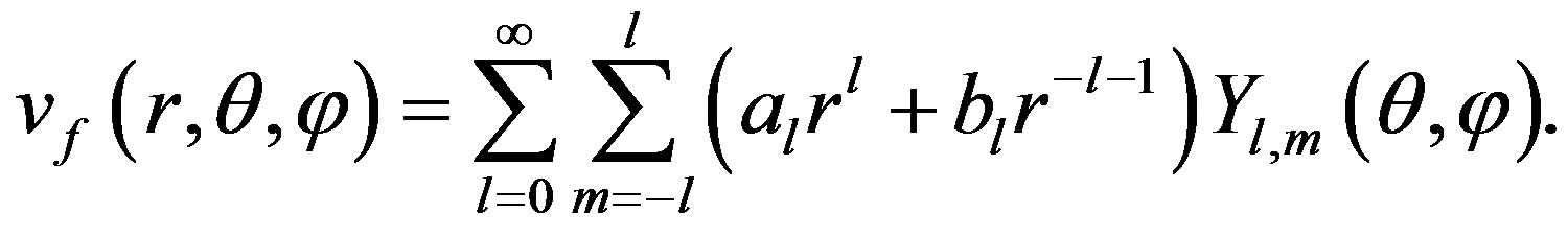 (7)
(7)
Therefore, we need to calculate the coefficients of (7) from the condition boundaries. Indeed, since the radius of points of  are equal to constant
 , then the condition boundary on
  implies easily, by identification, the following system:
But, on the boundary , the radius aren’t equal, and depend of spherical angle
 . Then, for this reason, we use Gauss-Ostrogradski theorem’s, whose we show that it is useful to find another relation between the coefficients of (7) like
 . Consequently, we get for each
 , a system of two equations with two unknowns
  and
and , which it is sufficient to calculate
  and
and :
:
Proposition 3.2. The condition boundary on  implies:
 (8)
(8)
Proof. Let , we construct the following vector field
  by:
by:
 (9)
(9)
whose,  is a primitive relative to
  for the following function:
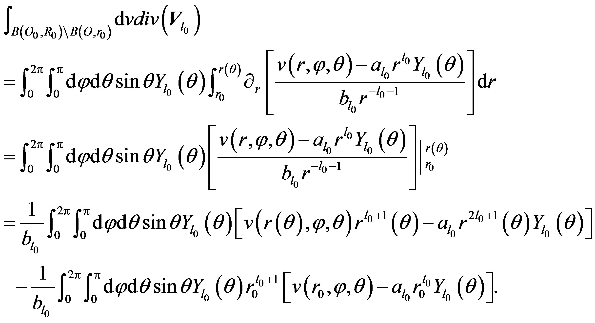
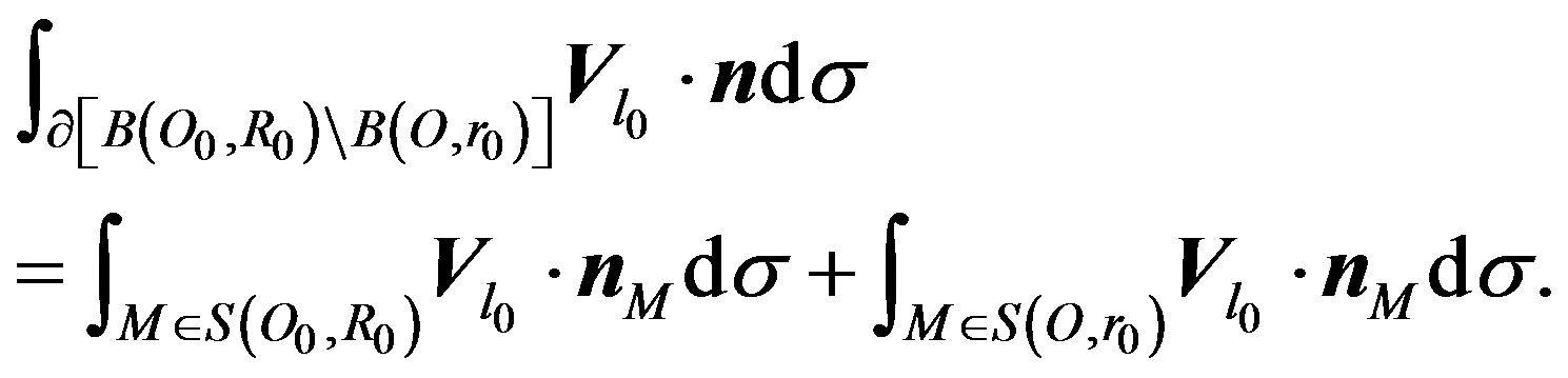
Calculate the flux of field  across the domain
  using Gauss-Ostrogradski theorem 3.1:
 (10)
(10)
where:
1. Calculate :
:
In domain , we have:

On the other hand,  can be calculated from (9) by:

Then, we deduce that:

Therefore, from Fubini’s theorem of multiple integrals, we obtain:
 (11)
(11)
Moreover, condition boundary on  implies that:

So, by replacing  by its value
  in (11), we deduce:
 (12)
(12)
But, we can prove that:
 (13)
(13)
Indeed: from (7), we have that

Multiplying by  the previous equation, and integrating it on domain
 , we obtain:
 (14)
(14)
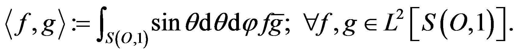
On the other hand, spherical harmonic functions form a basis for the Hilbert space  following inner product:
Consequently, we deduce, since
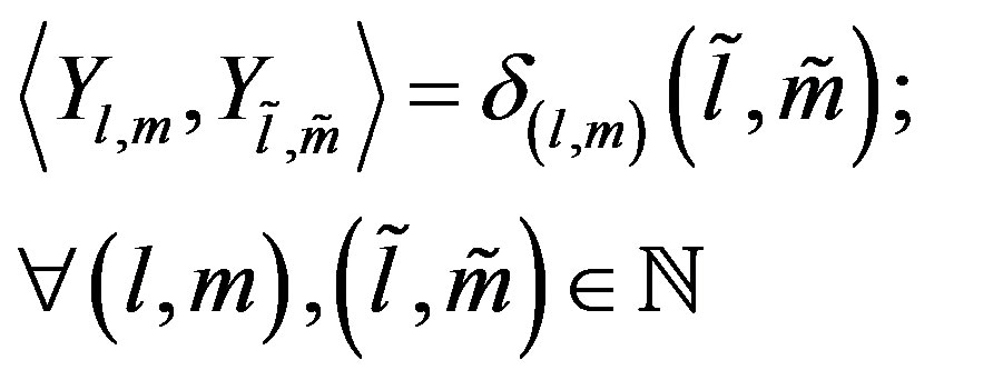 that:
that:
 (15)
(15)
Here,  designed Dirac function.
So, by inserting (15) in (14), we deduce above equality (13) as follows:
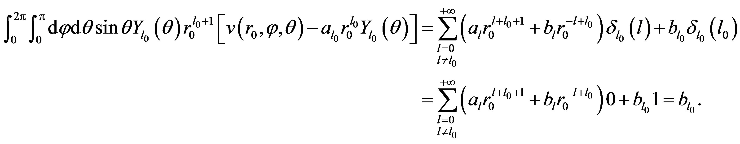
We continue the proof by inserting (13) in (12):
 (16)
(16)
2. Calculate :
:
knowing that,
 then:
then:
 (17)
(17)
2.1 Showing that:
 (18)
(18)
Indeed: unit outer-normal vector  relative to domain
  at arbitrary point
  is
is . This implies:
2.2 Showing that:
 (19)
(19)
Indeed: the symmetry of the shape implies that unit outer-normal vector of  relative to domain
  is below in plan generated by the two vectors
  and
and  which are orthogonal to field vector
  directed by
 . So, we obtain:
 .
.
Then, by inserting (18) and (19) in (9), we deduce that:
 (20)
(20)
3. Boundary Equation Finally, by inserting (16) and (20) in (10), we obtain that:

The previous equation ends the proof since it is true for any .
. 
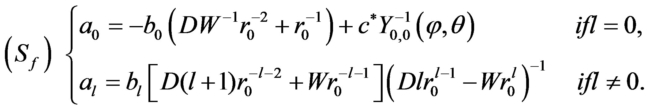
Proposition 3.3. If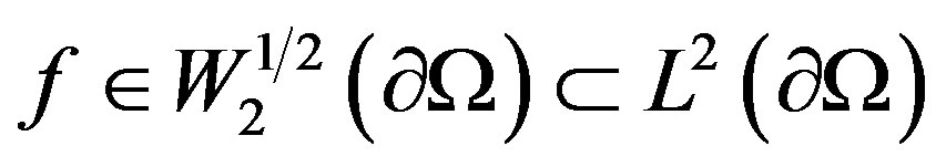 , then problem (P1) have unique solution with the form (7), whose the coefficients are given by:
• 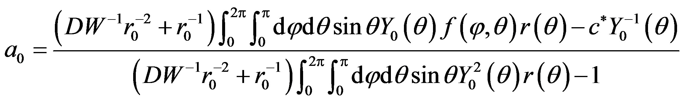
• 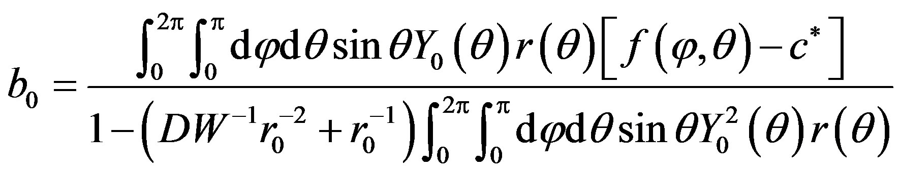
• 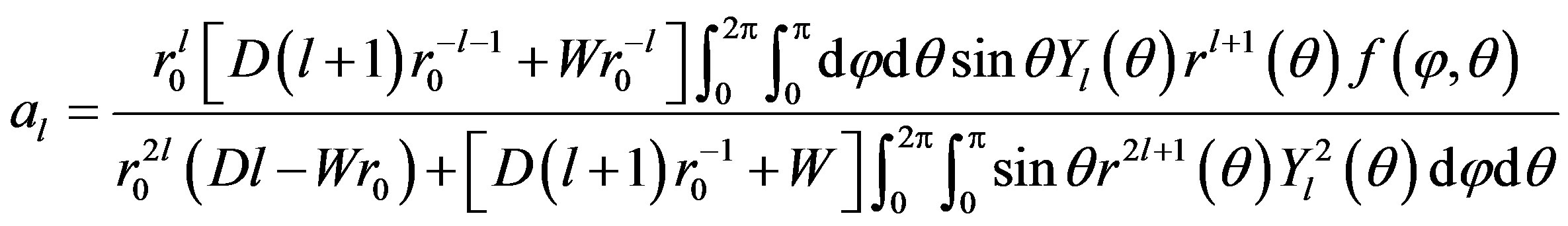
•  .
.
where,  is the distance
  between arbitrary point
  on sphere
 and the center
 .
.
Proof. It is enough to resolve for any , the system of two unknowns
  et
et  given by the two boundary conditions (8) and
 .
. 
Since the solution of problem (P1) is given from proposition 3.3, then we can deduce its relative Dirichletto-Neumann operator:
Corollary 3.4. The Dirichlet-to-Neumann operator (1) is defined by
 (21)
(21)
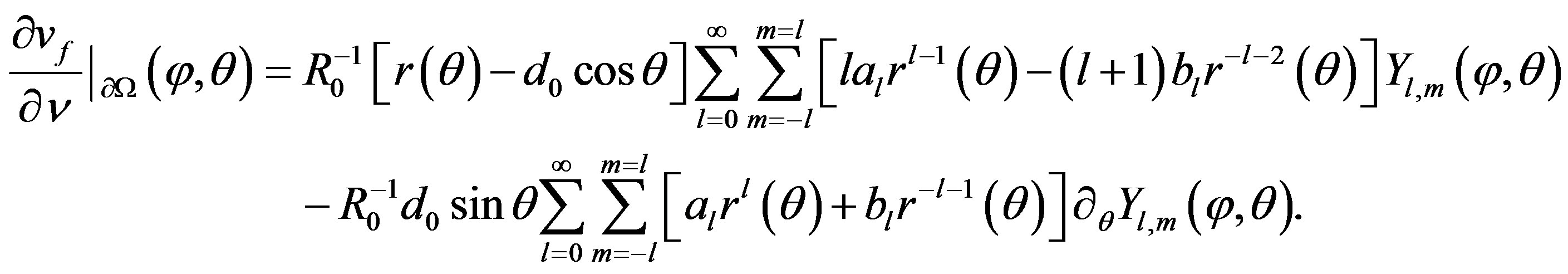
Here, the coefficients  are given by proposition 3.3.
Proof. Since we have that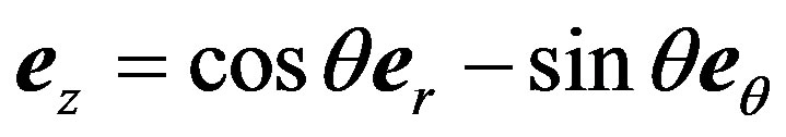 , then unit outer-normal vector
  for arbitrary point
  is given by:

and consequently, this implies:

But, we have from the proof of proposition 3.2 that . Then:

Consequently, it is enough to replace  in the previous equation by its value given in (7).
Remark 2. For general properties of Dirichlet-toNeumann operators, mainly existence and uniqueness, we refer to [10], chapter 4.
Remark 3. Notice that definition of Dirichlet-toNeumann operator (21) implies that it has as eigenfunctions the spherical harmonic function , and a discrete spectrum
 , whose
 .
.
Corollary 3.5. Dirichlet-to-Neumann operator (21) is unbounded, non-negative, self-adjoint, first-order elliptic pseudo-differential operator with compact resolvent on the Hilbert space .
.
Proof. For the proof, we refer to [10], chapter 4. 
Remark 4. Corollary 3.4 implies using Hille-Yosida’s theorem that Dirichlet-to-Neumann operator (21) can be generate certain semigroup . Moreover, we can prove using Arzela-Ascoli’s criterion that this semigroup is contractant holomorphic in the both Banach space
  and
and .
.
Proof. For a complete proof, see [10], chapter 4. 
4. Localisation Inverse Problem
We are interested by resolving the localisation inverse problem of (P1) using the explicit formula of , which will be calculated in terms of measurable Dirichlet-toNeumann boundary hypothesis on external boundary
 .
.
For resolving this problem, we need the following:
i) First, we aim to calculate the total flux  across external boundary
 .
.
ii) Second, we aim to find an equation involving the distance  between
  center of cell
  and
and
 center of
 .
.
Proposition 4.1. The total flux  and
and  satisfy the following:
 (22)
(22)
Proof. Since the differential element at the boundary  and unit outer-normal vector
  at arbitrary point
  are respectively equal to
  and
and , then we deduce from (7) that:
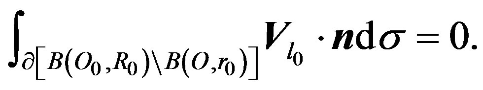
On the other hand, by Gauss-Ostrogradsky theorem, one gets:
where  is the volume differential element. Therefore, (22) is deduced.
Since we have, from proposition 4.1, that total flux  across external boundary
  depended only of one coefficient
  of development (7), whose
  depended of distance
 , then an equation of
  can be find easily. Indeed:
Corollary 4.2. The distance  verifies the following equation:
 (23)
(23)
Proof. It is enough to insert (22) in the expression of  given in proposition 3.2 in order to substitute
 , after replacing
  by its value in term of
 :
:
Consequently, the fact that  ends the proof.
5. Conclusions
(23) is an equation of the only unknown  involving the parameters
  and
and , which are the Dirichlet-to-Neumann hypothesis of problem (P1) on the external boundary, and we can found them from an experimental measures.
To summarize, we have found an equation for  which is the distance between the center
  of the cell
  and the center
  of
of , so it remains to find the position of the center
 . In fact:
Let  and
and  be two points at the external boundary
  whose the norm of the local current
  reaches respectively its maximum and minimum values, see Figure 1. Then, from the symmetry of the shape, we deduce that the center
  of the cell
  is localized at the line passed by the points
 ,
,  and
and , exactly between
  and
and  where the distance
  between
  and
and  is given by Equation (23).
By conclusion, we can now answer the question posed in the introduction about the uniqueness of the inverse localisation problem for (P1), and we can conclude that total flux  (2), involving Dirihlet-to-Neumann operator (1), is sufficient to resolve the localisation inverse problem, in three-dimensional case, if the shape is regular. But, it is not enough in other type of inverse problem like geometrical inverse problem, see [5].
6. Acknowledgements
I want to thank the CNRS Federation “Francilienne de
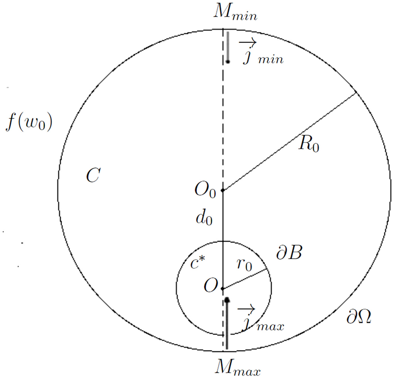
Figure 1. Position of the cell overline B.
Mecanique, Materiaux Structures et Procedes” CNRS FR2609, in particularly Prof. Didier Clouteau, for financial support in this study
REFERENCES
- J. Lee and G. Uhlmann, Communications on Pure and Applied Mathematics, Vol. 42, 1989, pp. 1097-1112. doi:10.1002/cpa.3160420804
- B. Sapoval, Physical Review Letters, Vol. 73, 1994, pp. 3314-3316. doi:10.1103/PhysRevLett.73.3314
- D. S. Grebenkov, M. Filoche and B. Sapoval, Physical Revie E, Vol. 73, 2006, Article ID: 021103. doi:10.1103/PhysRevE.73.021103
- O. Kellog, “Foundation of Potential Theory,” Dover, New York, 1954.
- I. Baydoun and V. A. Zagrebnov, Theoretical and Mathematical Physics, Vol. 168, 2011, pp. 1180-1191. doi:10.1007/s11232-011-0097-8
- I. Baydoun, Journal of Modern Physics, 2013, in Press, Article ID: 7501125.
- M. E. Taylor, “Partial Differential Equations II: Qualitative Studies of Linear Equations,” Springer-Verlag, Berlin, 1996. doi:10.1007/978-1-4757-4187-2
- J. K. Hunter and B. Nachtergaele, “Applied Analysis,” World Scientific, Singapore, 2001.
- D. Tataru, Communications in Partial Differential Equations, Vol. 20, 1995, pp. 855-884. doi:10.1080/03605309508821117
- I. Baydoun, Operateurs de Dirichlet-Neumann et leurs applications. Editions universitaires europeennes. 978- 3-417-9078-1, 2012.