Applied Mathematics
Vol.5 No.2(2014), Article ID:42173,9 pages DOI:10.4236/am.2014.52032
On Metaheuristic Optimization Motivated by the Immune System
1Department of Mathematics, Faculty of Science, King Khalid University, Abha, KSA
2Department of Mathematics, Faculty of Science, Mansoura University, Mansoura, Egypt
Email: *mohfathy@mans.edu.eg
Received November 16, 2013; revised December 16, 2013; accepted December 23, 2013
ABSTRACT
In this paper, we modify the general-purpose heuristic method called extremal optimization. We compare our results with the results of Boettcher and Percus [1]. Then, some multiobjective optimization problems are solved by using methods motivated by the immune system.
Keywords:Multiobjective Optimization; Extremal Optimization; Immunememory and Metaheuristic
1. Introduction
Multiobjective optimization problems (MOPs) [2] are existing in many situations in nature. Most realistic optimization problems require the simultaneous optimization of more than one objective function. In this case, it is unlikely that the different objectives would be optimized by the same alternative parameter choices. Hence, some trade-off between the criteria is needed to ensure a satisfactory problem. Multiobjective (Multicriteria) optimization has its roots in late 19th century welfare economics, in the works of Edge worth and Pareto. A mathematical description is as follows: finding the vector  which satisfies the
  inequality constraints
 , the p equality constraints
 , and minimizing the vector function
 , where
 , is the vector of decision variables, each decision variable xi
 ![]() is bounded by lower and upper limits
is bounded by lower and upper limits . The space in which the objective vector belongs is called the objective space and the image of the feasible set under F is called the attained set.
The scalar concept of optimality does not apply directly in the multiobjective setting. A useful replacement is the notion of Pareto optimality. So, we have the following definitions related to this notation [3]:
Definition 1 (Pareto dominance) A vector  is said to be dominated by another vector
  iff
iff .
.
Definition 2 (Pareto optimality) A solution ![]() is said to be Pareto optimal with respect to Ω
is said to be Pareto optimal with respect to Ω ![]() iff; there is no
iff; there is no  for which
  dominate
 .
.
Pareto optimal points are also known as efficient solutions, non-dominated, or non-inferior points.
Definition 3 (Pareto optimal set) The Pareto optimal set  is the set of Pareto optimal solutions, i.e.
 .
.
Definition 4 (Pareto optimal front) The Pareto optimal front  is the set of objective functions values corresponding to the solutions in
 , i.e.
 .
.
The multiobjective problem is almost always solved by combining the multiple objectives into one scalar objective whose solution is a Pareto optimal point for the original MOP. Most algorithms have been developed in the linear framework (i.e. linear objectives and linear constraints), but the techniques described below are also applicable to nonlinear problems. Several methods have been proposed to solve continuous multiobjective optimization problems. In the next section, some multiobjective methods are discussed. In the third section, extremal optimization is introduced and two immune motivated optimization algorithms are proposed. In Section 4, we generalize extremal optimization to multiobjective optimization.
2. Some Multiobjective Optimization Methods
Almost every real life problem is multiobjective problem [2,4]. Methods for solving multiobjective optimization problems are mostly intuitive. Here, we list and discuss some of them.
The first method is the Minimizing Weighted Sums of Functions. A standard technique for MOP is to minimize a positively weighted convex sum of the objectives , that is,
  where
where  and
and .
.
It is known that the minimizer of this combined function is Pareto optimal. It is up to the user to choose appropriate weights. Until recently, considerations of computational expense forced users to restrict themselves toper forming only one such minimization. Newer, more ambitious approaches aim to minimize convex sums of the objectives for various settings of the convex weights, therefore generating various points in the Pareto set. Though computationally more expensive, this approach gives an idea of the shape of the Pareto surface and provides the user with more information about the trade-off among the various objectives. However, this method suffers from two drawbacks. First, the relationship between the vector of weights and the Pareto curve is such that a uniform spread of weight parameters rarely produces a uniform spread of points on the Pareto set. Often, all the points found are clustered in certain parts of the Pareto set with no point in the interesting/middle part" of the set, thereby providing little insight into the shape of the trade-off curve. The second drawback is that non-convex parts of the Pareto set cannot be obtained by minimizing convex combinations of the objectives (note though that non-convex Pareto sets are seldom found in actual applications).
Here another problem is considered. Assume that the set  of decisions weights
  reflecting decision-makers’ preferences. A matrix
  is obtained after asking the decision maker to quantify the ratio of his/her preferences of one decision over another. In other words, for every pair of decisions
 , the term
  is requested satisfying
 , i.e. instead of giving the weights
 ![]() directly, he/she has a matrix A. This matrix must be a positive reciprocal matrix, i.e.
directly, he/she has a matrix A. This matrix must be a positive reciprocal matrix, i.e. . For a given positive reciprocal matrix A, different procedures can be followed in order to obtain weights
 . By Perron-Frobenius theorem [5], the matrix A has a unique positive dominant eigenvalue. But due to the above properties of
 ![]() one can derive the following:
one can derive the following:
Proposition 1 If , then the eigenvalues of A in the case of n objectives are n; 0 where the zero is repeated
 ![]() times.
times.
Proof: It is direct to see that the characteristic polynomial of the positive reciprocal matrix A satisfies the recurrence relation;
 (1)
(1)
And .
.
Using mathematical induction the proposition is proved.
Now, there are two simple methods to determine the weights  given the matrix A [6]. The first method is that the required weights are proportional to the eigenvector corresponding the unique eigenvalue n by solving
![]() , where
, where  is the weight vector. The second method is that it is proportional to the row geometric mean of
 ![]() i.e. they are given by;
i.e. they are given by; .
.
It has been argued that the method of weighted sums of objectives is one of the best methods in multiobjective combinatorial optimization (MOCO) [7]. The reason is that Pareto set for discrete variables is a set of points. Such set can be obtained via a convex combination of the objectives e.g. the weights method.
The second method is the Homotopy Techniques. Homotopy techniques aim to trace the complete Pareto curve in the bi-objective case (n = 2). By tracing the full curve, they overcome the sampling deficiencies of the weighted sum approach [8,9]. The main drawback is that this approach does not generalize to the case of more than two objectives.
The third method is the Goal Programming. In the goal programming approach, we minimize one objective while constraining the remaining objectives to be less than given target values e.g. minimize  subject to
 , where
  are parameters to be gradually decreased till no solution is found. This method is especially useful if the user can afford to solve just one optimization problem. However, it is not always easy to choose appropriate goals for the constraints
 . Goal programming cannot be used to generate the Pareto set effectively, particularly if the number of objectives is greater than two.
The fourth method is Multilevel Programming. Multilevel programming is a one-shot optimization technique and is intended to find just one optimal point as opposed to the entire Pareto surface. The first step in multilevel programming involves ordering the objectives in terms of importance. Next, we find the set of points ![]() for which the minimum value of the first objective function
for which the minimum value of the first objective function  is attained. We then find the points in this set that minimize the second most important objective
 . The method proceeds recursively until all objectives have been optimized on successively smaller sets. Multilevel programming is a useful approach if the hierarchical order among the objectives is of prime importance and the user is not interested in the continuous trade-off among the functions. However, problems lower down in the hierarchy become very tightly constrained and often become numerically infeasible, so that the less important objectives have no influence on the final result. Hence, multilevel programming should surely be avoided by users who desire a sensible compromise solution among the various objectives. Also, this method is called lexicographic method.
A famous application is in university admittance where students with highest grades are allowed in any college they choose. The second best group is allowed only the remaining places and so on. The drawback of this method is that two distinct lexicographic optimization with distinct sequences of the same objective functions does not produce the same solution. Also, this method is useful but in some cases it is not applicable.
A fifth method using fuzzy logic is to study each objective individually and find its maximum and minimum say ,
,  respectively. Then determine a membership
 . Thus
![]() .
.
Then apply . Again this method is guaranteed to give a Pareto optimal solution. This method is a bit difficult to apply for large number of objectives.
A sixth method is the Keeney-Raiffa method which uses the product of objective functions to build an equivalent single objective one called Keeney-Raiffa utility function.
The seventh method is Normal-Boundary Intersection [10,11]. The normal-boundary intersection method (NBI) uses a geometrically intuitive parameterization to produce an even spread of points on the Pareto surface, giving an accurate picture of the whole surface. Even for poorly scaled problems (for which the relative scaling on the objectives are vastly different), the spread of Pareto points remains uniform. Given any point generated by NBI, it is usually possible to find a set of weights such that this point minimizes a weighted sum of objectives, as described above. Similarly, it is usually possible to define a goal programming problem for which the NBI point is a solution. NBI can also handle problems where the Pareto surface is discontinuous or non-smooth, unlike homotopy techniques. Unfortunately, a point generated by NBI may not be a Pareto point if the boundary of the attained set in the objective space containing the Pareto points is non-convex or “folded” (which happens rarely in problems arising from actual applications). NBI requires the individual minimizers of the individual functions at the outset, which can also be viewed as a drawback.
3. Extremal Optimization and the Immune System
In this section, we concentrate more on extremal optimization then relate it to the immune system and generalize it to multiobjective cases.
Extremal Optimization (EO) is an optimization heuristic inspired by the Bak-Sneppen model of self-organized criticality from the field of statistical physics [1,12]. This heuristic was designed initially to address combinatorial optimization problems such as the travelling salesman problem and spin glasses, although the technique has been demonstrated to function in optimization domains. EO was designed as a local search algorithm for combinatorial optimization problems. Unlike genetic algorithms, which work with a population of candidate solutions, EO evolves a single solution and makes local modifications to the worst components. This requires that a suitable representation be selected which permits individual solution components to be assigned a quality measure (“fitness”). This differs from holistic approaches such as ant colony optimization and evolutionary computation that assign equal-fitness to all components of a solution based upon their collective evaluation against an objective function. The algorithm is initialized with an initial solution, which can be constructed randomly, or derived from another search process.
In the Bak-Sneppen model, species are located on the sites of a lattice, and have an associated fitness value between 0 and 1. At each time step, the one species with the smallest value (poorest degree of adaptation) is selected for a random update, having its fitness replaced by a new value drawn randomly from a flat distribution on the interval [0; 1]. But the change in fitness of one species impacts the fitness of interrelated species. Therefore, all of the species at neighboring lattice sites have their fitness replaced with new random numbers as well. After a sufficient number of steps, the system reaches a highly correlated state known as self-organized criticality [13].
Extremal optimization is quite similar to the way the immune system (IS) renews its cells [14]. Almost everyday new immune cells are replaced in the blood stream. If within few weeks they were able to recognize antigens (viruses or bacteria) then they are preserved for longer period. Otherwise they are replaced randomly. This dynamics is called extremal dynamics (EO) [15]. It can explain the long range memory of the immune system even without the persistence of antigens. The reason is that if a system evolves according to such dynamics then the annihilation probability for a clone (a type of cells) that has already survived for time t is inversely proportional to , where c is a constant. Boettcher and Percus [1] have used extremal optimization to solve some single objective combinatorial optimization problems. Their algorithm have been modified by [12,16] and used to solve 3-dimensional spin glass and graph coloring problems.
Definition 5 Extremally driven systems are the systems that updated by identifying an active region of the system and renewing this region whilst leaving the remainder unchanged. The active subsystem is chosen according to some kind of extremal criterion; often it is centered on the location of the minimum of some spatially varying scalar variable.
Consider a system of n elements, each element assigned a single scalar variable  drawn from the fixed probability distribution function
 . For every time step, the element with the smallest value in the system is selected and renewed by assigning a new value which is drawn from
 . It is assumed that no two
  can take the same value.
Definition 6 For the above system the typical values of  increase monotonically in time. This means that any renewed element is likely to have a smaller
  than the bulk, and hence a shorter than average lifespan until it is again renewed. Corresponding, elements that have not been renewed for sometime will have a longer than average life expectancy. This separation between the shortest and the longest lived elements will become more pronounced as the system evolves and the average
  in the bulk increases. This phenomenon is called long-time memory.
Proposition 2 Extremally driven systems can generally be expected to exhibit long-term memory [15].
Proof Let  be the probability to find the system in a state S after t updates, where
 . At the next step
 ![]() only one of the values will change that may be any one of the
only one of the values will change that may be any one of the ![]() elements. Let
elements. Let  be the state that
  is the smallest value. Then
  can be given by,
 , (2)
, (2)
where the function  is defined by;
 . (3)
. (3)
Using the substitution , Equation (2) can be rewritten as;
 , (4)
, (4)
where ,
,  and
and
 .
.
Identity 1 Since  and
and  are independent, then;
 . (5)
. (5)
Identity 2 , (6)
, (6)
Where  is the domain of space in which
  is the smallest, and
 .
.
Now, let us return to Equation (4), using identity (1) and , we can get;


 .
.
Then;
 (7)
(7)
Since ![]() is symmetric in
is symmetric in  and therefore in
 , the probability that any particular element in the systemsay
![]() , is the smallest at a given time
, is the smallest at a given time  is
is . Let
. Let  is the probability to find the system in a state Sat a time
  given that
 ![]() was not the minimum at any of the times
was not the minimum at any of the times , then;
 . (8)
. (8)
The corresponding probability that ![]() is the smallest, denoted by
is the smallest, denoted by  can be calculated by integrated Equation (8) over
  using Equation (6);
 , (9)
, (9)
which independent of  also
also . Then the probability of an element being renewed decreases with the time since it was last renewed according to
 , also
 .
.
 is defined as the probability that a randomly chosen element
 ![]() has the same value of
has the same value of  at time
that it had at![]() , then
, then  and
and . For
. For ![]() observe that
observe that  only decrease when an element is renewed for the first time, so
  hence from Equation (9);
 . (10)
Since ,
,  , then
 . (11)
The slow decay of  shows that a significant proportion of the system will remain in its initial state until arbitrarily late times, already suggesting some form of long-term memory.
The existence of aging can be most clearly expressed in terms of the two-time correlation function  between the state of the system at times
  and
and . The probability that a randomly chosen element has the same value of
  at times
  and
and  is
is . Note that
 ,
,
 where
where ,
,

 .
.
After a short transient this scales as .
.
That t and  only appear in the ratio
  is what we mean by aging. Aging indicates the existence of some form of long-term memory. Finally, as N tends to infinity we get
  and
and
 where
where . This can explain the long term memory of the immune system in the absence of antigens.
Nature has been created in a fascinating way. As we learn more, we found that it is more efficient to imitate it. Recently, this approach has been applied to optimization [1]. The author’s considered the spin glass problem. They assign a spin variable  for each site
 . Each site is connected to each nearest neighbors
  via a bond variable
 , assigned at random. The goal is to find the configuration
 , to approximately minimize the cost function or Hamiltonian;
 . (12)
Also, they assigned a fitness  to each spin variable xi
 ![]() by the relation
by the relation . Then the one with the lowest fitness is removed and replaced with another one at random. It has been applied to the both, spin glass and graph coloring problems. The extremal optimization algorithm is as follows:
Choose  randomly to form an initial configuration
![]() , set
, set . Repeat the following steps as desired1) Find the fitness
  of the variable
  for all
 .
.
2) Find the site  with the lowest fitness (i.e.
 ) and choose another configuration
 ![]() randomly such that
randomly such that  is replaced by another state.
3) If  then
then , else
 .
.
The weakness of this approach is that focusing only on the worst fitness can lead to narrow deterministic process. To overcome this weakness, the authors replaced step (2) of the above algorithm by ranking the sites in an ascending order according to their fitness. Then the replaced site is chosen randomly according to the probability distribution .
.
We proposed two modifications. The first immune motivated optimization IMOP1 replaces the second step (2) by the following1) Find the fitness  of the variable
  for all
 .
.
2) Replace randomly the sites with lowest 5% fitness (not just the one with the lowest fitness).
3) If  then
then , else
 .
.
This gives a significantly higher fitness than the previous deterministic one (at the same time) but still it has the previous drawback of falling in local minima. The second immune motivated optimization algorithm IMOP2 which preserves the advantage of the above modification is to define ![]() by;
by;
 , (13)
Where  is the maximum (minimum) possible fitness and
![]() . The second step in the above algorithm IMOP1 is now replaced by the following1) Find the fitness
. The second step in the above algorithm IMOP1 is now replaced by the following1) Find the fitness  of the variable
  for all
 .
.
2) For all , if
, if  then replace
 .
.
3) If  then
then , else
 .
.
where RND is a uniformly distributed random number. This algorithm has the following advantages1) It has a better chance of avoiding getting stuck in local minima.
2) It does not require the ranking of all fitness at each time step as the modification of Boettcher and Percus requires. This saves significant time especially for large number of sites.
We reconsidered the spin glass problem (that Boettcher studied in his paper [1]) and apply our immune motivated optimization algorithm IMOP2. We graphed the average energies obtained by Boettcher and that obtained by our algorithm for the ±J spin glass in  as a function of τ. For each
 , where L is the length of the cube, 10 instances were chosen. For each instance 10 runs were performed stating from different initial conditions at each
 . The results were averaged over the number of runs and over the number of instances. We can see from the figures (from Figures 1(a) to (d) for
![]() ,
, ![]() ,
, ![]() and
and  and from the results of Boettcher that we get better minimum values than them in all case. Also, we can see from Figures 2 and 3, that we reach to better minimum values in the same time that Boettcher’s takes. This means that our approach is faster than the ordinary EO.
In Table 1, we compare the modified EO approximations to the average ground-state energy per spin  of the ±J spin glass in
  with EO results using Extremal optimization. For each size
  we have studied a large number
  of instances. Also shown is the average time
  (in seconds) needed for EO to find the presumed ground state. We note that the new results are better and faster than the other three results.
4. Extremal Optimization as a Multiobjective Metaheuristic
Generalizing extremal optimization to multiobjective optimization is done by defining the weighted fitness at
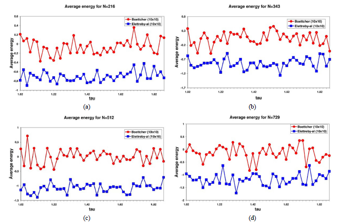
Figure 1. (a-d) Plot of the average energies obtained by EO (red) and modified EO forthe ±J spin glass in d = 3 as a function of τ for size n =216, 343, 512, 729.
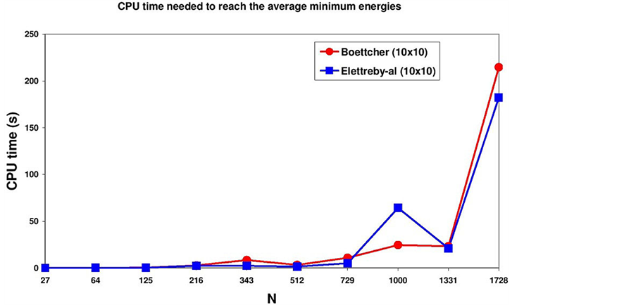
Figure 2. This figure shows the time needed to reach the minimal average energy for each L. The red line is our results using modified EO algorithm and the blue one is the results using.
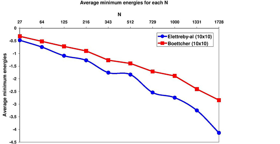
Figure 3. This figure shows the minimal average energy for each L. The red line is our results using modified EO algorithm and the blue one is the results using.

Table 1. Shows a comparison between the modified EO results, EO results.
each site by,
 , where
 ,
, . (14)
Then we apply the extremal optimization algorithm.
Now, we comment on extremal optimization as a metaheuristic optimization procedure.
Definition 7. A metaheuristic [17] is an iterative process which guides a heuristic by learning strategies to find a near optimal solution.
Metaheuristics are characterized by:
1) They give approximate solutions.
2) They include mechanisms to avoid being trapped into locally optimal solutions.
3) They are not a specific problem.
4) They include diversified and intensified mechanisms for an efficient search of solutions.
Extremal optimization has all these properties. The intensification and diversification mechanisms are included in the random number in the algorithm IMOP2. If the random number is large, a large number of sites are going to change their state hence diversification occurs. If the random number is small, only a small number of sites will change their state hence intensification occurs.
REFERENCES
- S. Boettcher and A. Percus, “Optimization with Extremal Dynamics,” Physical Review Letters, Vol. 86, No. 23, 2001, pp. 5211-5214.
- Y. Collette and P. Siarry, “Multi-Objective Optimization: Principles and Case Studies,” Springer, New York, 2003.
- M. R. Chen and Y. Z. Lu, “A Novel Elitist Multiobjective Optimization Algorithm: Multiobjective Extremal Optimization,” European Journal of Operational Research, Vol. 188, No. 3, 2008, pp. 637-651. http://dx.doi.org/10.1016/j.ejor.2007.05.008
- M. Ehrgott, “Multi-Criteria Optimization,” Springer, New York, 2005.
- N. F. Britton, “Essential Mathematical Biology,” Springer, New York, 2003. http://dx.doi.org/10.1007/978-1-4471-0049-2
- R. Blanquero, E. Carrizosa and E. Conde, “Inferring Efficient Weights from Pairwise Comparison Matrices,” Mathematical Methods of Operations Research, Vol. 64, No. 2, 2006, pp. 271-284. http://dx.doi.org/10.1007/s00186-006-0077-1
- I. Das, “Applicability of Existing Continuous Methods in Determining Pareto Set for a Nonlinear Mixed Integer Multicriteria Optimization Problem,” 8th AIAA Symposium on Multidiscipline, Analysis and Optimization, Longbeach CA, 2000. http://dx.doi.org/10.2514/6.2000-4894
- J. R. Rao and P. Y. Papalambros, “A Non-Linear Programming Continuation Strategy for One Parameter Design Optimization Problems,” In: B. Ravani, Ed., Advances in Design Automation Montreal, Vol. 19, No. 2, Que, Canada, 17-21 September 1989, ASME, New York, pp. 77-89.
- J. Rakowska, R. T. Haftka and L. T. Watson, “Tracing the Efficient Curve for Multi-Objective Control-Structure Optimization,” Computing Systems in Engineering, Vol. 2, No. 6, 1991, pp. 461-471. http://dx.doi.org/10.1016/0956-0521(91)90049-B
- I. Das and J. E. Dennis, “Normal-Boundary Intersection: A New Method for Generating the Pareto Surface in Nonlinear Multicriteria Optimization Problems,” SIAM Journal on Optimization, Vol. 8, No. 3, 1998, pp. 631-657. http://dx.doi.org/10.1137/S1052623496307510
- I. Das, “Nonlinear Multicriteria Optimization and Robust Optimality,” Ph.D., Department of Computational and Applied Mathematics, Rice University, Houston, 1997.
- E. Ahmed and M. El-Alem, “Immune Motivated Optimization,” International Journal of Theoretical Physics, Vol. 41, No. 5, 2002, pp. 985-990. http://dx.doi.org/10.1023/A:1015705512186
- P. Bak and K. Sneppen, “Punctuated Equilibrium and Criticality in a Simple Model of Evolution,” Physical Review Letters, Vol. 71, No. 24, 1993, pp. 40834086. http://dx.doi.org/10.1103/PhysRevLett.71.4083
- I. Roitt and P. Delves, “Essential Immunology,” Blackwell Publishers, 2001.
- D. Head, “Extremal Driving as a Mechanism for Generating Long-Term Memory,” Journal of Physics A: Mathematical and General, Vol. 33, No. 42, 2000, p. L387. http://dx.doi.org/10.1088/0305-4470/33/42/102
- E. Ahmed and M. F. Elettreby, “On Combinatorial Optimization Motivated by Biology,” Applied Mathematics and Computation, Vol. 172, No. 1, 2006, p. 4048. http://dx.doi.org/10.1016/j.amc.2005.01.122
- C. Blum and A. Roli, “Metaheuristics in Combinatorial Optimization: Overview and Conceptual Comparison,” ACM Computing Survey, Vol. 35, No. 3, 2003, pp. 268-308.
NOTES

*Corresponding author.