ABSTRACT

We extend a recently proposed Quantum Field Theory (QFT) approach to the Lifshitz formula, originally implemented for a real scalar field, to the case of a fluctuating vacuum Electromagnetic (EM) field, coupled to two flat, parallel mirrors. The general result is presented in terms of the invariants of the vacuum polarization tensors due to the media on each mirror. We consider mirrors that have small widths, with the zero-width limit as a particular case. We apply the latter to models involving graphene sheets, obtaining results which are consistent with previous ones.

1. Introduction

Lifshitz’ formula [1], provides a quite useful tool for the evaluation of the Casimir force [2] between bodies with parallel planar interfaces, and rather arbitrary frequencydependent dielectric functions. In its original version, two disjoint media-filled half-spaces with plane, parallel boundaries were considered; the calculation was performed at finite temperature, and the final result for the interaction force was presented in terms of the dielectric functions that described, macroscopically, the electromagnetic properties of each media.

The successive refinements achieved in precision experiments measuring the Casimir force have provided a continuous stimulus to generalize the scope of the Lifshitz formula, in order to encompass either new or more realistic situations [3]. One of those generalizations has been considered models where the fluctuating vacuum field, rather than being subject to ideal, “sharp and strong” boundary conditions, is instead in the presence of background potentials, localized on the mirrors [4,5]. These potentials are meant to implement smooth versions of the perfect boundary conditions. A possible way to justify them is by resorting to the microscopic point of view. Indeed, by taking into account the interaction of the internal degrees of freedom on the mirrors with the fluctuating field [5,6], one may derive an approximate effective action for the vacuum field, containing potentials with support at the positions of the material slabs. Even assuming them, as we shall do throughout this paper, to have time independence and translation invariant properties along the two “parallel” directions, , the potentials are, in general, nonlocal functions of time as well as of and. The non locality in can be dealt with by a Fourier transformation in, since this yields a potential which is local in frequency as well as in the parallel components of the momentum. The resulting Fourier transformed potential will still carry a dependence on the normal coordinate, the direction along which the effect of the potential on the fluctuating field is strongest. The potential must be, then, necessarily non invariant under translations in. We shall nevertheless assume that its dependence on is local1.

In [8], a QFT approach was used to derive Lifshitz formula for a fluctuating real scalar field coupled to two material slabs, in a situation like the previously described one regarding both the geometry involved and the simplifying assumptions made. It is the aim of this article to adapt the approach of that reference to the case of a fluctuating Abelian gauge field. The derivation in [8] relied upon the application of the Gelfand-Yaglom (G-Y) formula for functional determinants [9] (for a modern review, see [10]), objects which arise quite naturally within the path integral formulation, for example, when incorporating corrections due to fluctuations, in the presence a nontrivial background.

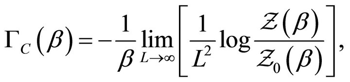
Although we shall mostly deal with zero temperature calculations, it is convenient, for the sake of generality, to formulate the problem in terms of the Casimir free energy per unit area,. This may, in turn, be obtained from the partition function:

(1)

where is a length that characterizes the size of the plates. can be written as an Euclidean functional integral:

(2)

where is the Euclidean action for the gauge field, including its coupling to the mirrors. The integral over the time-like Euclidean coordinate is understood to be taken over a finite interval of length, with periodic boundary conditions for the field. The spatial coordinates are assumed to be confined to a box of side length, with Dirichlet boundary conditions2.

Since we shall be interested in the Casimir force, we discard factors independent of, the distance between the mirrors. That is represented in (1) by the division by, which denotes the partition function when the mirrors are infinitely far apart.

Relevant physical observables shall be the vacuum energy per unit area, as well as the Casimir force per unit area,:

(3)

and its zero-temperature limit.

In this article, we derive expressions for as a function of the invariants that define the vacuum polarization tensor for the media on the mirrors, as well as of the “shape” of the mirrors, understanding by that the specific form of the dependence of those tensors. We do that for (finite) small-width mirrors and for zerowidth mirrors, as an important special case of the former. In both cases we consider, we take advantage of the fact that the problem is essentially one-dimensional, and that it can be reduced to a collection of scalar problems. For them, we apply G-Y theorem for its exact evaluation.

This paper is organized as follows: in Section 2 we introduce the class of model that we shall consider, writing the partition function in terms of the physical objects that define the system: the positions and shapes of the mirrors and their vacuum polarization tensors. Then in Section 3, we transform the system into two one-dimensional scalar problems.

In 4, we start from the partition function and show that it can be so transformed as to be evaluated using the results of [8]. We then present the corresponding Lifshitz formula.

The Casimir effect for systems involving graphene sheets has been recently studied in a series of interesting papers ([11-13]), including thermal effects. In Section 5 we apply the general formula to that kind of system as a consistency check, deriving an explicit expression for cases involving graphene mirrors as a function of the parameters defining the vacuum polarization tensor. In Section 6 we present our conclusions.

2. The Model

Throughout this article, we consider models where the EM field is coupled to two imperfect mirrors modeled by “potentials” which are local in and translation invariant in. Note, however, that those potentials, since they couple to the gauge field, will also have a tensor structure.

As in the approach of [8], we define the system in terms of its Euclidean action,. Denoting by the Abelian gauge field, that action may be written as follows:

(4)

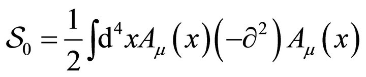
where denotes the free gauge field action and the term that accounts for the coupling to the mirrors. The former has the standard form:

(5)

with the gauge invariant piece:

(6)

and for the gauge-fixing term we assume the form:, with being a positive real constant.

The interaction action is assumed to be composed of two terms, each one describing the interaction between and a mirror:

(7)

, will be assumed to describe the interaction with a single mirror, whose properties are time independent as well as homogeneous and isotropic on each plane. Regarding the direction (normal to both mirrors), we assume the properties of the mirrors to be local functions of that coordinate.

Besides, we use the fact that the interaction terms preserve gauge invariance. This is guaranteed, if the current due to the charged microscopic degrees of freedom which induce the coupling terms is conserved. Finally, the coupling terms are assumed to be quadratic in, which is a reasonable assumption to make when one deals with media that may be appropriately described by linear response theory.

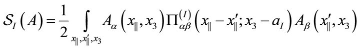
Then may be put into a more explicit form: using a shorthand notation for the integrations, and assuming the mirror to be centered at, we may write the term that describes its interaction with the gauge field as follows:

(8)

where is the vacuum polarization tensor, i.e., the correlator between currents, for the matter fields on the mirror.

Equation (8) suggests the consideration of two situations, the second a particular case of the first, regarding the mirror’s extent along the normal coordinate. Firstly, we may regard it to have small width, in the sense that the charge carriers in the medium are strongly concentrated in a finite region. Since there is no current along, the vacuum polarization tensor (a correlator between currents) will be zero when one or two of its indices equals 3. Secondly, we shall deal with the zero-width limit of the previous case.

Here, the currents are essentially planar, and we shall then neglect the action of on the third component of the gauge field.

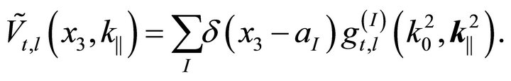
Thus, in the small width case we shall have,

(9)

where is the vacuum polarization tensor for the medium confined to the mirror. A convention we use is that in (9), and run from to. This implies that the mirrors shall only involve the parallel components of the electric field, and the normal component of the magnetic field,.

The tensor, is assumed to be, as a function of, concentrated on a region centered around. Note that we are not assuming that necessarily can be written as the product of a function of by a function of,. For the case of very thin slabs, like the ones we shall consider when dealing with graphene-like mirrors, that factorization is a natural assumption to make. However, one could consider vacuum polarization tensors which properties depends non trivially on the normal coordinate.

Performing a partial Fourier transformation in (9), i.e., just for the time and the parallel coordinates, we see that:

(10)

Here, and in what follows, we use the notation. We implicitly assume that the component is summed over discrete values,

(the Matsubara frequencies) at finite temperature, and integrated (continuum values) at zero temperature.

We have thus set up the general structure of the kind of systems that we shall consider here. In the next section we show how to decompose the problem of evaluating for the gauge field into two independent one-dimensional systems, each one corresponding to a single real scalar field.

3. Reduction to One-Dimensional Systems

Thus each mirror has been characterized by its vacuum polarization tensor. It is convenient to decompose each one of them in terms of scalar functions, something that can be achieved, for example, by expanding the tensor into a complete set of orthogonal projectors. That decomposition is rather general, since it can be obtained as a consequence of the assumptions we have made.

Let us first note that, current conservation of the charge carriers in the media implies that, for each, the tensor is transverse, namely:

(11)

Regarding the condition above, we can find two independent solutions to the transversality condition, so that may be decomposed into two irreducible transverse tensors (projectors), in terms of two scalars. Indeed, the assumed isotropy and homogeneity of the media along the parallel directions, means that we can construct two independent transverse tensors using as building blocks the elements:, and, where. Note that the presence of is allowed since Poincaré invariance on the spacetime does not hold necessarily true.

Two independent projectors and that are solutions of (11) may be written as follows:

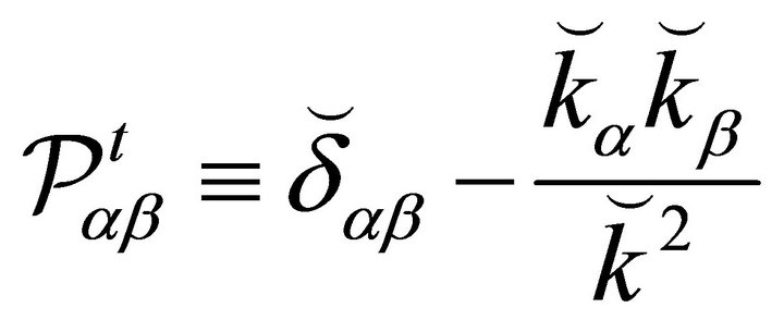(12)

and

(13)

where

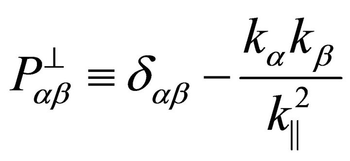(14)

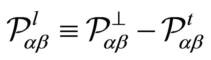
is the transverse projector corresponding to a dimensional Poincaré covariant theory. For the sake of completeness, we also introduce the ‘parallel’ projector:

(15)

They satisfy the following algebraic properties:

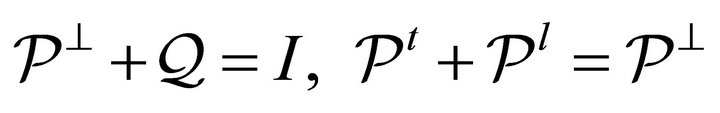
(16)

where. Therefore we can express as follows:

(17)

In this way, we have succeeded in characterizing the mirror by two functions,. To proceed to the reduction of the problem of evaluating to onedimensional functional determinants, we shall perform the same Fourier transformation we used for the interaction terms, for the free action. Adopting the Feynman gauge choice,

(18)

we see that

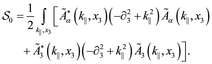(19)

Then, the complete action may be split into two terms, one depending on and the other on:

(20)

with:

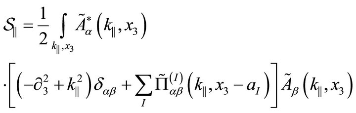(21)

and

(22)

Note that, because of (20), and the fact that does not involve any coupling to the mirrors, we may write the ratio between and as follows:

(23)

with:

(24)

Applying the properties satisfied by the projectors, we see that:

(25)

which allows us to write:

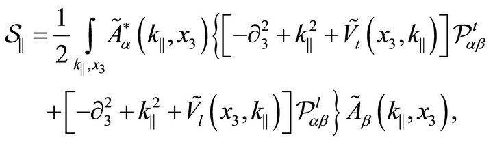(26)

where

(27)

what concludes the reduction. Indeed, note that the action has been reduced to a quadratic form for an operator which has been decomposed into orthogonal rank-one projectors.

4. Lifshitz Formula

To obtain the Lifshitz formula for this kind of model, we proceed as follows: In the path integral for, we may decompose the gauge field:

(28)

under which the path integral measure factorizes. Thus,

(29)

where each factor is obtained as the result of performing a functional integral over one scalar degree of freedom, namely,

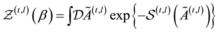(30)

where

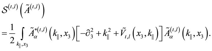(31)

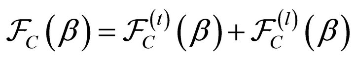
Then we see that the free energy becomes:

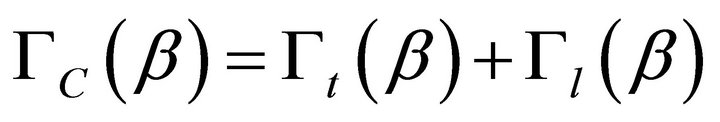(32)

where

(33)

or

(34)

where:

(35)

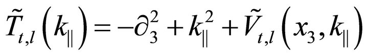
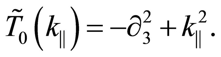
The system has been reduced to two independent Casimir problems, each one of them corresponding to a real scalar field in the presence of its potential background. These potentials are built in terms of the functions that appear in the decomposition of the vacuum polarization tensor into a set of irreducible tensors.

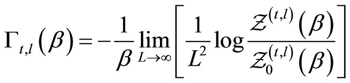
Applying the general formula derived in [8], we may write for each contribution above:

(36)

where is the result of performing the following change of basis to the matrix:

(37)

with

(38)

and are defined as in [8], regarding each one, or, as due to an independent field, in its own background potential.

5. Zero Width Mirrors

We characterize thin mirrors here as systems where the interaction between field and mirrors is confined to zero-width planes. Thus, in this case,

(39)

and

(40)

Recalling the known result of [8] for the case of a real scalar field in the presence of zero width mirrors, we see that:

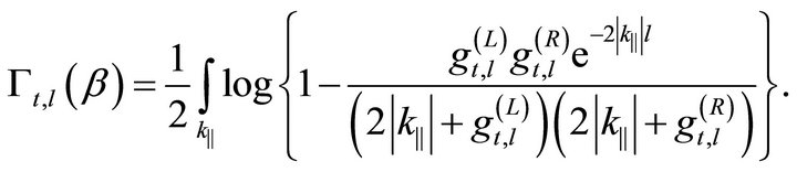(41)

Then, the Casimir force per unit area becomes:

(42)

with

(43)

where the arguments of and were omitted.

For a graphene sheet ([11-13]), which can be reasonably described by a zero-width mirror, the corresponding functions may be read off from its vacuum polarization tensor, the result being:

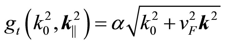
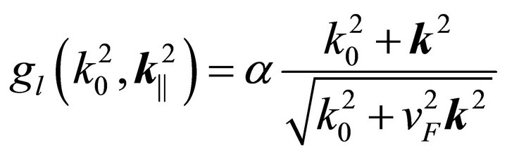(44)

with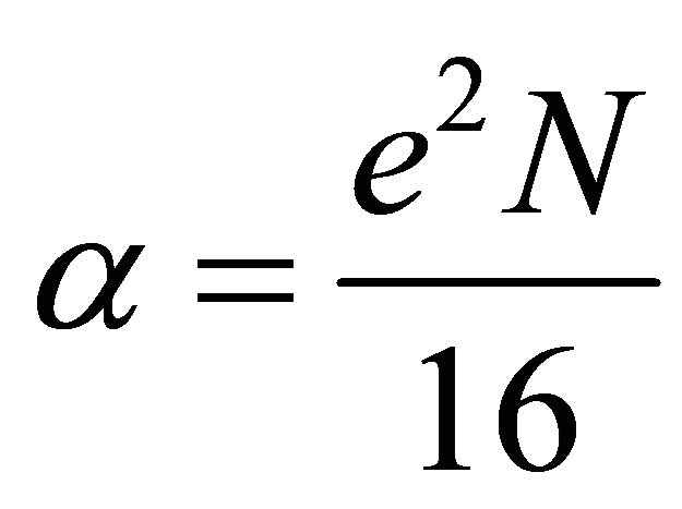, where is the number of fermion flavours, the couppling constant, and the Fermi velocity.

Using these expressions into the general formula for thin mirrors, we obtain the Casimir force for cases involving either two graphene sheets or, as a limiting case, a graphene sheet and a conducting mirror. The latter may be obtained from the graphene case by setting the Fermi velocity to 1 and in one of the mirrors.

In Figure 1 we plot the zero temperature pressure times as a function of for the case of a perfectly conducting mirror in front of a graphene sheet, for different values of, and in Figure 2 for two identical graphene sheets. Note that in both figures the solid line corresponding to represents a ‘relativistic matter’ case, where, considered in [6].

6. Conclusions

We have derived a general expression for the Casimir free energy, using an entirely field theoretic approach, whereby the problem is analyzed in terms of the functional determinant for a fluctuating Abelian gauge field. We have shown that, under some assumptions regarding form of the coupling between the gauge field and the mirrors, the problem can be reduced to scalar systems,

for which one can apply the previously known expression for the functional determinant.

The result is expressed in terms of the invariants of the Euclidean version of the vacuum polarization tensor due to the charged matter inside the mirror. In this way one may bypass the calculation of the reflection coefficients of each mirror, as it would be the case with the usual version of Lifshitz formula. Besides, the result for smallwidth mirrors allows for cases where the material media have a non trivial dependence along the normal direction; for example, one could consider vacuum polarization tensors corresponding to stratified media.

For zero width mirrors with graphene like properties, we have shown that the QFT approach yields results which are consistent with the ones presented in [11-13].

7. Acknowledgements

This work was supported by CONICET, and UNCuyo.

REFERENCES

NOTES

¹Non localities along the normal coordinate can be incorporated, for example, in an approach like the one of [7].

²The final result, for, shall be insensitive to the choice of boundary conditions on that spatial box.

REFERENCES

- E. M. Lifshitz, “The Theory of Molecular Attractive Forces between Solids,” Sov. Phys. JETP, Vol. 2, 1956, pp. 73-83.
- H. B. G. Casimir, “On the Attraction between Two Perfectly Conducting Plates,” Indagationes Mathematicae, Vol. 10, 1948, pp. 261-263; Koninklijke Nederlandse Akademie van Wetenschappen Proceedings, Vol. 51, 1948, pp. 793-795; Frontiers of Physics, Vol. 65, 1987, pp. 342-344; Koninklijke Nederlandse Akademie van Wetenschappen Proceedings, Vol. 100, No. 3-4, 1997, pp. 61- 63.
- P. W. Milonni, “The Quantum Vacuum: An Introduction to Quantum Electrodynamics,” Academic Press, San Diego, 1994.
- N. Graham, R. L. Jaffe, V. Khemani, M. Quandt, O. Schroeder and H. Weigel, “The Dirichlet Casimir Problem,” Nuclear Physics B, Vol. 677, No. 1-2 2004, pp. 379-404. doi:10.1016/j.nuclphysb.2003.11.001
- C. D. Fosco, F. C. Lombardo and F. D. Mazzitelli, “Casimir Energies with Finite-Width Mirrors,” Physical Review D, Vol. 77, 2008, pp. 085018 1-12.
- C. D. Fosco, F. C. Lombardo and F. D. Mazzitelli, “Casimir Effect with Dynamical Matter on Thin Mirrors,” Physics Letters B, Vol. 669, No. 5, 2008, pp. 371-375. doi:10.1016/j.physletb.2008.10.004
- C. D. Fosco and E. Losada, “Casimir Effect with Nonlocal Boundary Interactions,” Physics Letters B, Vol. 675, No. 2, 2009, pp. 252-256. doi:10.1016/j.physletb.2009.03.084
- C. Ccapa Ttira, C. D. Fosco and F. D. Mazzitelli, “Lifshitz Formula for the Casimir Force and the GelfandYaglom Theorem,” Journal of Physics A, Vol. 44, 2011, pp. 465403 1-13.
- I. M. Gelfand and A. M. Yaglom, “Integration in Functional Spaces and It Applications in Quantum Physics,” Journal of Mathematical Physics, Vol. 1, No. 1, 1960, pp. 48-69. doi:10.1063/1.1703636
- G. V. Dunne, “Functional Determinants in Quantum Field Theory,” Journal of Physics A, Vol. 41, 2008, pp. 304006 1-15.
- M. Bordag, B. Geyer, G. L. Klimchitskaya and V. M. Mostepanenko, “Lifshitz-Type Formulas for Graphene and Single-Wall Carbon Nanotubes: Van der Waals and Casimir Interactions,” Physical Review B, Vol. 74, 2006, pp. 205431 1-9.
- M. Bordag, I. V. Fialkovsky, D. M. Gitman and D. V. Vassilevich, “Casimir Interaction between a Perfect Conductor and Graphene Described by the Dirac Model,” Physical Review B, Vol. 80, 2009, pp. 245406 1-5.
- I. V. Fialkovsky, V. N. Marachevsky and D. V. Vassilevich, “Finite Temperature Casimir Effect for Graphene,” Physical Review B, Vol. 84, 2011, pp. 035446 1-13.
NOTES
1Non localities along the normal coordinate can be incorporated, for example, in an approach like the one of [7].
2The final result, for , shall be insensitive to the choice of boundary conditions on that spatial box.