Applied Mathematics
Vol.4 No.1A(2013), Article ID:27502,7 pages DOI:10.4236/am.2013.41A036
Automatic Simulation of the Chemical Langevin Equation
Department of Mathematics, Ryerson University, Toronto, Canada
Email: *silvana@ryerson.ca
Received November 20, 2012; revised December 27, 2012; accepted January 4, 2013
Keywords: Stochastic Biochemical Kinetics; Chemical Langevin Equation; Derivative-Free Milstein Method
ABSTRACT
Biochemical systems have important practical applications, in particular to understanding critical intra-cellular processes. Often biochemical kinetic models represent cellular processes as systems of chemical reactions, traditionally modeled by the deterministic reaction rate equations. In the cellular environment, many biological processes are inherently stochastic. The stochastic fluctuations due to the presence of some low molecular populations may have a great impact on the biochemical system behavior. Then, stochastic models are required for an accurate description of the system dynamics. An important stochastic model of biochemical kinetics is the Chemical Langevin Equation. In this work, we provide a numerical method for approximating the solution of the Chemical Langevin Equation, namely the derivative-free Milstein scheme. The method is compared with the widely used strategy for this class of problems, the Milstein method. As opposed to the Milstein scheme, the proposed strategy has the advantage that it does not require the calculation of exact derivatives, while having the same strong order of accuracy as the Milstein scheme. Therefore it may be used for an automatic simulation of the numerical solution of the Chemical Langevin Equation. The tests on several models of practical interest show that our method performs very well.
1. Introduction
A fundamental problem in the post-genomic biology is to describe and analyze the complex dynamical interactions which take place at the level of a single cell. Recent experimental techniques made it possible to study gene regulatory networks in living cells [1] as well as to generate synthetic gene networks [2].
There are currently several levels of refinement used for modeling the cellular dynamics. Often chemical kinetic models represent cellular processes as systems of chemical reactions. Traditionally, these processes were modeled as continuous deterministic systems, by reaction rate equations. However, the random fluctuations which are captured by the experiments [3-6] are neglected by such models. These fluctuations are due to low molecular numbers of some biochemical species. Then, stochastic models are required for an accurate description of the system dynamics. A stochastic model of the well-stirred biochemical systems is the Chemical Master Equation [7]. Various algorithms proposed for the exact simulation of the solution of the Chemical Master Equation [8,9] are computationally very expensive for most practical applications. Approximate algorithms were designed and analyzed in the literature to speed-up the simulation for biochemical systems modeled with the Chemical Master Equation [10-14]. Nonetheless, more sophisticated techniques are necessary for dealing with systems which manifest stiffness. Stiffness is due to the presence of the multiple time-scales in the system, as some reactions are much faster than others.
As an intermediate model between the Chemical Master Equation and the reaction rate equations, the Chemical Langevin Equation (CLE) [15] is considered a very attractive choice in modeling many important biological processes. CLE consists of a system of stochastic differential equations, nonlinear and with non-commutative multiplicative noise. Most biochemical systems of interest typically involve many components interconnected in a complex manner. Thus, it is important to have efficient and accurate algorithms for simulating their mathematical models and in particular if they are stiff. However, the construction of algorithms to simulate and approximate the solution to these mathematical models is a challenging task, and research in this field is only at the initial stages [16-18]. One of the widely used numerical methods to simulate the Chemical Langevin Equation is the Milstein scheme [19,20]. This scheme has strong order of accuracy one, however it necessitates the calculation of some exact derivatives. This is a drawback of the Milstein strategy.
This paper provides a derivative-free numerical method for the strong approximation of the solution of the Chemical Langevin Equation. To our knowledge, the derivative-free Milstein scheme was not utilized before in the simulation of stochastic models of biochemical kinetics. The advantages of this method include: it is of strong order of accuracy one and it does not entail the calculation of exact derivatives. The derivative-free Milstein strategy estimates the derivatives by using finite differences. The proposed method may therefore be used for designing automatic simulation algorithms for generic models of well-stirred biochemical systems, in the Langevin regime.
The paper is organized as follows. Section 2 gives an introduction to the strong numerical solution of Itô stochastic differential equations. In Section 3 we discuss a stochastic continuous model of well-stirred biochemical kinetics, namely the Chemical Langevin Equation. Section 4 presents our proposed numerical strategy for the Chemical Langevin Equation. Numerical tests on several models of practical interest, showing the accuracy of the method provided, are given in Section 5. Finally, we summarize our conclusions in Section 6.
2. Background
A brief introduction to the numerical solution of Itô stochastic differential equations (SDE), which are essential in stochastic biochemical kinetic modelling, is presented below. The Itô formulation of an SDE system is
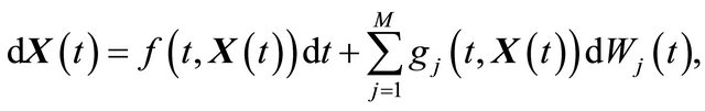 (1)
(1)
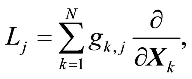
where X is an N-dimensional stochastic process. Here  and
and  are N-dimensional and represent the drift and the diffusion coefficients, respectively, while
  denotes an M-dimensional Wiener process with independent components.
We are interested in the strong numerical solution of SDE. Strong numerical approximations are employed when an accurate approximation of the solution of an SDE on individual trajectories is desired, while weak numerical approximations are utilized when the approximation of the moments of the exact solution is sufficient.
Let XL be the numerical approximation on [0, T], after L steps with stepsize , of the exact solution
  of (1) and let
  be a constant.
2.1. Strong Convergence
The approximation  of
of  is said to have strong order of convergence γ if there exists a constant
 , independent of h and
 , such that the following is true
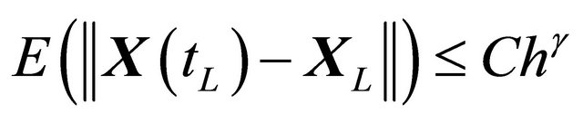 (2)
(2)
for any .
.
2.2. Weak Convergence
The approximation  of
of  is said to have weak order of convergence γ if, for any polynomial P there exists a constant
 , independent of h and
 , such that
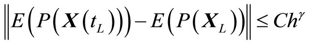 (3)
(3)
for any .
.
Here  denotes the expectation of a random variable and
  a norm of an N-dimensional vector.
The focus of this work is on SDE with non-commutative noise [20], as the Chemical Langevin Equation has multiplicative non-commutative noise. For this class of problems, to obtain numerical methods of strong order of accuracy 1 on each interval , in addition to the computation of the Wiener increments
with , the simulation of the stochastic double Itô integrals
  is necessary or, equivalently, of the Levy areas. The double Itô integrals
  are defined as
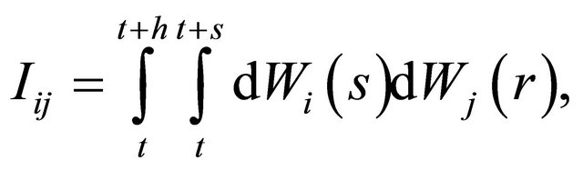
for any .
.
The double Itô integrals are estimated in terms of their Fourier series expansion truncated after p terms (see also [20]):
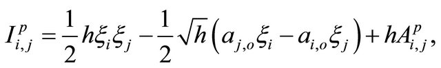
where, for any ,
,
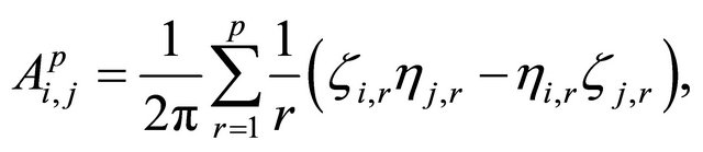
and
with
The random variables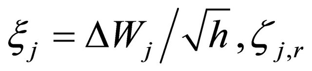 and
and 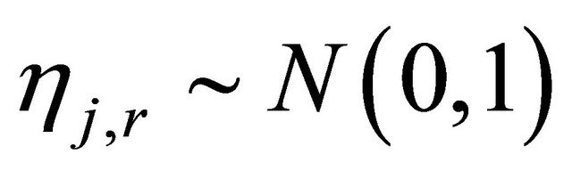 are independent normally distributed with mean 0 and variance 1, for any
  and any
 . Numerical experiments in the literature indicate that
 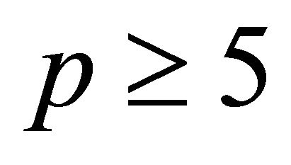 is sufficient for an accurate approximation
  of the double Itô integrals
 . In our simulations we choose p = 5.
2.3. Milstein Method
The classical strong order 1 numerical method due to Milstein is used in the literature for approximating the exact solution of the Chemical Langevin Equation [19]. The Milstein scheme on the time interval  is given by
 (4)
(4)
where the Wiener increments are denoted by 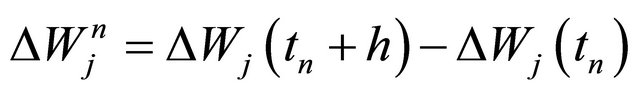 .
.
The differential operator  is defined as
 (5)
(5)
for any .
.
2.4. Derivative-Free Milstein Method
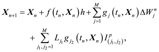
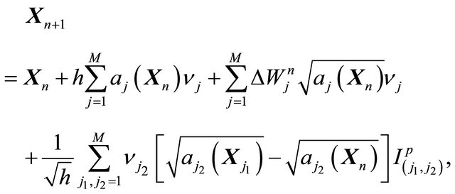
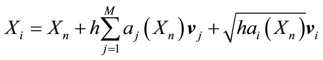
The strong order 1 Milstein strategy has the disadvantage that it requires derivative calculations, an issue for generating automatic simulation algorithms. The derivativefree Milstein schemes [21] overcome this difficulty. The derivative-free Milstein strategy for the general SDE (1), driven by M independent Wiener processes can be obtained from the Milstein method by replacing the derivatives by finite differences. Note that these differences require intermediate approximations at other points. The derivative-free Milstein scheme can be written as
 (6)
(6)
where the intermediate values are
 (7)
(7)
for .
.
3. Stochastic Continuous Models of Biochemical Kinetics
It has recently been acknowledged that stochastic models are more accurate than their deterministic counterparts for representing cellular dynamics. Biological processes at the single cell level are often modeled as systems of biochemical reactions. Below we discuss a key stochastic model of well-stirred biochemical kinetics. This model is valid for isothermal biochemically reacting systems with relatively large molecular numbers, in a constant volume.
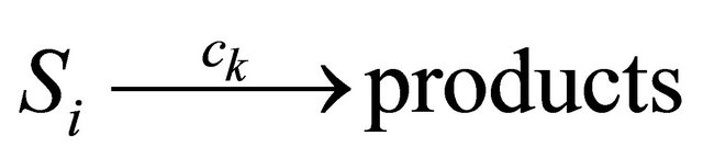
Assume that N biochemical species  undergo M reaction channels
 . The well-stirred assumption leads to a simplification of the molecular dynamics model. Under the above assumptions, the system state can be represented by a stochastic process
 . The components of the dynamical state vector are
 , the number of molecules of the
  species present in the system at time t, for any
 .
.
Each reaction  is completely characterized by its propensity and its state-change vector. The state-change vector of the reaction
 , is an N-dimensional vector with the component
  being the variation in the number of molecules of the
  species produced by the firing of one reaction
 . The matrix
is the stoichiometric matrix of the biochemical system.
The propensity  of the reaction
  is defined as
  is the probability that a single reaction
  occurs in the time-interval
 , given the state x at time t. The existence of the propensity function is a consequence of the kinetic theory.
A unimolecular reaction
has propensity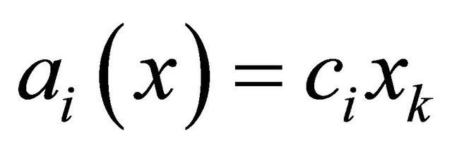 . The bimolecular reaction

is characterized by the propensity 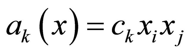 if
if  and by the propensity
  if
if  (the reaction being called dimerization).
Assume that the system has a macroscopic time-scale. More precisely, we assume that a time step h exists satisfying simultaneously the conditions.
1) h is small enough such that no propensity varies significantly in the interval ,
,
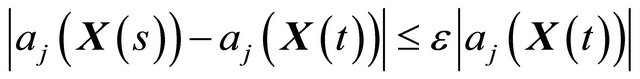 (8)
(8)
for  and each
 .
.
2) and h is large enough such that each reaction  occurs many times in the time-interval
  or, equivalently, for any
 (9)
(9)
The conditions 1) and 2) are satisfied for biochemical systems with abundant molecular numbers. Then, the dynamical state of the system may be approximated by a continuous Markov process  satisfying
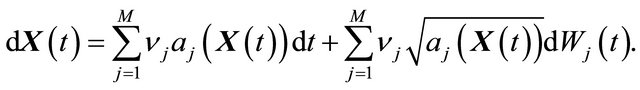 (10)
(10)
Here  denote independent Wiener processes. The Equation (10) is called the Chemical Langevin Equation (CLE) and it is a system of non-commutative Itô SDE. The SDE (10) has an associated Fokker-Planck equation [15], a partial differential equation which governs the probability density of the dynamical state
 . The dynamical state
  is required to obey the initial condition
 (11)
(11)
at .
.
4. Derivative-Free Simulation of the Chemical Langevin Equation
In this paper we propose to utilize the derivative-free Milstein strategy for simulating the Chemical Langevin Equation. The derivative-free Milstein scheme has strong order of accuracy 1 as the Milstein method, but achieves it without making use of exact derivatives. The computation of the exact derivative required by the Milstein technique constitutes a difficulty for designing automatic simulating algorithms for the CLE, as it necessitates the user's input of the expression of the exact derivative. The method we propose for the CLE avoids this problem.
The Chemical Langevin Equation (10) is a particular case of the SDE (1), with the drift coefficient
 (12)
(12)
and the diffusion coefficients
 (13)
(13)
for .
.
The derivative-free Milstein method applied to the CLE (10) is derived by substituting the drift and diffusion coefficients (12) and (13), respectively, in the scheme (6) to get
 (14)
(14)
on the time-interval . The approximations at the intermediate points are
 (15)
(15)
for .
.
In the next section we test this method by comparing it to the Milstein scheme for the CLE as well as with Gillespie’s algorithm [8,9], on some models of biochemical systems of interest in applications.
5. Numerical Experiments
Below are presented numerical tests of our proposed method for approximating the solution of the Chemical Langevin Equation of a generic model of biochemical systems. The simulations are performed in Matlab [22]. The numerical strategy proposed is tested on several models of biochemically reaction systems arising in applications. We compare our method with the Milstein method, which is typically employed for simulating the CLE. However, there is no known biochemical system for which the Chemical Langevin Equation model has a closed form solution. To validate the accuracy of our numerical strategy we compare the histogram obtained with our method with the one computed with Gillespie’s algorithm [8,9]. Gillespie’s algorithm is a Monte Carlo simulation strategy which generates trajectories in exact accordance with the probability distribution of the Chemical Master Equation. The Chemical Langevin Equation model is an approximation of the Chemical Master Equation model, valid in the regime of large molecular population numbers. While there is also a modeling error when comparing the histograms generated with our method for the CLE and with Gillespie’s algorithm for the Chemical Master Equation, we note that the agreement of the numerical results is excellent, thus our scheme is shown to be very accurate.
5.1. Michaelis-Menten Model
Consider the Michaelis-Menten model [23], which deals with a very important mechanism of enzymatic catalysis. Four molecular species are involved in three reactions
 (16)
(16)
The species S1 is a substrate, S2 is an enzyme, S3 represents an enzyme-substrate complex, while S4 is a product. The biochemical model shows how the enzyme transforms the substrate into a product. The reaction rate parameters are 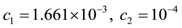 and
and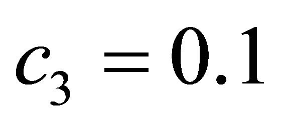 , while the propensity functions associated with the reactions (16) are
 (17)
(17)
The solution of the system (16) is subject to the initial conditions 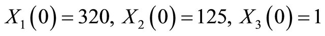 and
and 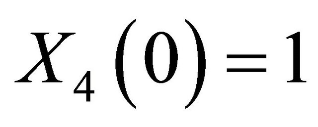 . The simulation is performed on the timeinterval [0, 30]. Finally, the state-change vectors are the columns of the following stoichiometric matrix
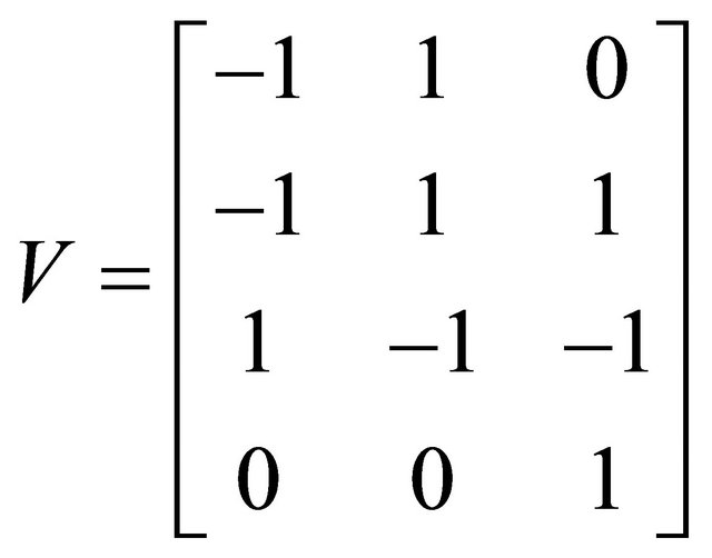
The simulations with the derivative-free Milstein method with stepsizes h1 = 10−1, h2 = 5 × 10⁻² and h3 = 10−1, with the Milstein scheme for the step h1 = 10−1 and with Gillespie’s algorithm are presented in Figure 1. Each integration is performed over 10,000 trajectories. We note that our method has a similar computational cost with the Milstein scheme. We computed the ratio of the execution time of the Milstein method and that of our derivative-free Milstein technique. The value of this ratio for the sequence of steps above is between 0.98 and 1.01, showing that the two methods have almost the same computational cost on this model. Figure 1 presents the histograms at t = 30 for the species S1, S2, S3, and S4, respectively. The accuracy of our method is excellent on this model.
5.2. Stiff Biochemical Model
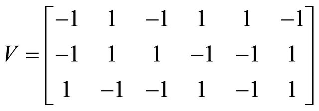
Below we illustrate our derivative-free scheme on a more complex system, a stiff non-linear biochemical model, consisting of the following reversible reactions
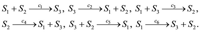
The reaction rate constants are  and c6 = 2. The system is integrated on the interval
 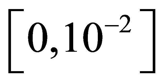 with initial conditions
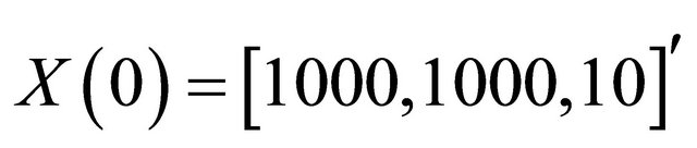 . The reactions above are characterized by the propensities
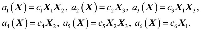 (18)
(18)
Also, the state-change vectors are the corresponding columns of the stoichiometric matrix
We ran the simulations for the proposed derivativefree Milstein, the Milstein and the Gillespie algorithms over 10,000 trajectories. The system is stiff as several orders of magnitude separate some of the propensities. As in the case of deterministic problems, in stochastic systems stiffness poses challenges to the numerical simulation. Our proposed method can integrate the system efficiently and accurately. Figure 2 shows the histograms computed at time 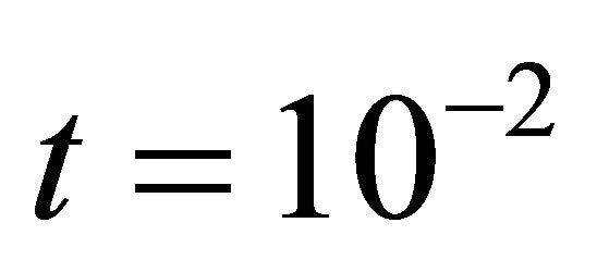 with the proposed derivative-free Milstein, Milstein and the Gillespie algorithms, respectively. We illustrate the behavior of our method applied with stepsize
  and compare it with the behavior of the Milstein strategy for the same step. The agreement between the results of the two numerical integrators is very good. We also study the be-
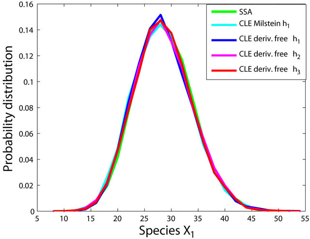
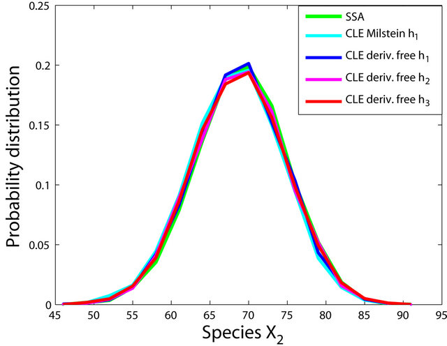
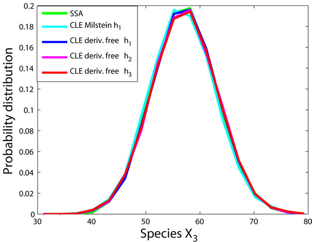
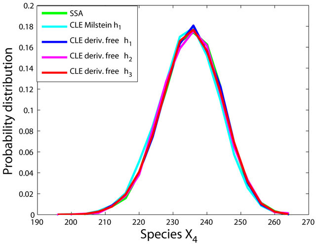
Figure 1. The Michaelis-Menten model: the histograms generated with the Gillespie algorithm, the Milstein method with step h1 = 10−1 and the derivative-free Milstein method with steps h1 = 10−1, h2 = 3 × 10⁻² and h3 = 10−2 at time t = 30 for the species S1, S2, S3 and S4 are shown. The simulation is over 10,000 trajectories.
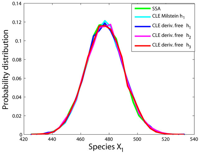
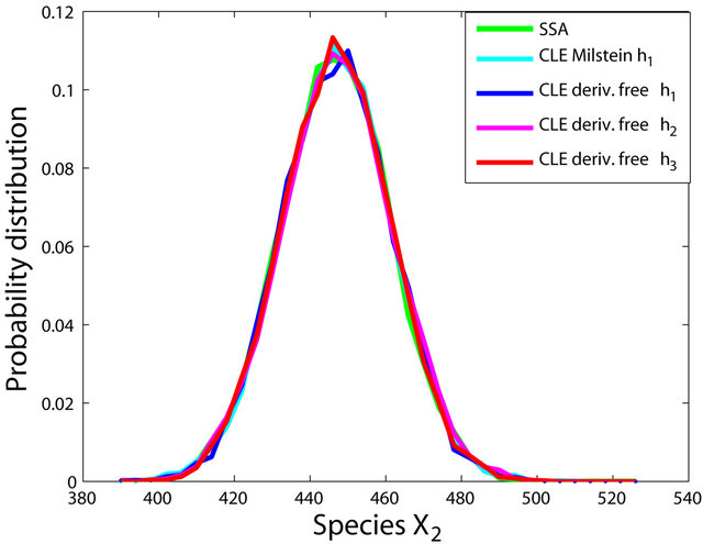
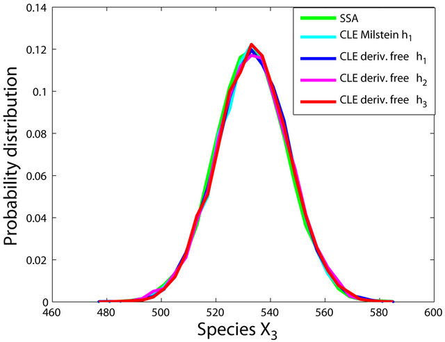
Figure 2. The stiff model: the histograms generated with the Gillespie algorithm, the Milstein method with step h1 = 10−5 and the derivative-free Milstein method with steps h1 = 10−5, h2 = 5 × 10⁻⁶ and h3 = 10−6 at time t = 10−2 for the species S1, S2 and S3 are plotted. The simulation uses 10,000 paths.
havior of our method for a sequence of time-steps h1 = 10−5, h2 = 5 × 10⁻⁶ and h3 = 10−6. As expected, the accuracy of our algorithm improves when the step is reduced. In addition, we computed the ratio of the execution times of the Milstein scheme and of the proposed derivative-free Milstein method for the steps above and found that the ratio ranges between 1.003 and 1.031, showing a very similar computational cost of the two methods. Finally, for the given sequence of time-steps the derivative free Milstein histogram matches closely that of the Gillespie’s algorithm, which shows that our method is very accurate.
The advantage of our derivative-free Milstein algorithm over the existing Milstein strategy is that ours can generate the numerical solution automatically, and does not require the user’s input regarding the computation of the exact derivatives, as the Milstein scheme does.
6. Conclusion
In this work we described the derivative-free Milstein method for approximating the solution of the Chemical Langevin Equation. Chemical Langevin Equation is a key model of well-stirred biochemical systems, with many important practical applications. Many models arising in practice are mathematically stiff and therefore their simulation may be quite challenging. The method we discuss in this paper achieves strong order of accuracy one as the Milstein scheme, which is currently the most widely used simulation technique for the Chemical Langevin Equation. Unlike the Milstein scheme, the method we provided above does not require the computation of exact derivatives, which is a drawback of the Milstein technique. The tests on key biochemical models arising in applications show the excellent accuracy of our method.
7. Acknowledgements
This work was supported in part by a grant from the Natural Sciences and Engineering Research Council of Canada (NSERC).
REFERENCES
- H. Kitano, “Computational Systems Biology,” Nature, Vol. 420, No. 6912, 2002, pp. 206-210. doi:10.1038/nature01254
- M. B. Elowitz and S. Leibler, “A Synthetic Oscillatory Network of Transcriptional Regulators,” Nature, Vol. 403, No. 6767, 2000, pp. 335-338. doi:10.1038/35002125
- A. P. Arkin, J. Ross and H. H. McAdams, “Stochastic Kinetic Analysis of Developmental Pathway Bifurcation in Phage-Infected Escherichia coli Cells,” Genetics, Vol. 149, 1998, pp. 1633-1648.
- W. J. Blake, M. Kaern, C. R. Cantor and J. J. Collins, “Noise in Eukaryotic Gene Expression,” Nature, Vol. 422, No. 6932, 2003, pp. 633-637. doi:10.1038/nature01546
- N. Federoff and W. Fontana, “Small Numbers of Big Molecules,” Science, Vol. 297, No. 5584, 2002, pp. 1129- 1131. doi:10.1126/science.1075988
- M. B. Elowitz, A. J. Levine, E. D. Siggia and P. S. Swain, “Stochastic Gene Expression in a Single Cell,” Science, Vol. 297, No. 5584, 2002, pp. 1183-1186. doi:10.1126/science.1070919
- D. T. Gillespie, “A Rigorous Derivation of the Chemical Master Equation,” Physica A, Vol. 188, No. 1-3, 1992, pp. 402-425. doi:10.1016/0378-4371(92)90283-V
- D. T. Gillespie, “A General Method for Numerically Simulating the Stochastic Time Evolution of Coupled Chemical Reactions,” Journal of Computational Physics, Vol. 22, No. 4, 1976, pp. 403-434. doi:10.1016/0021-9991(76)90041-3
- D. T. Gillespie, “Exact Stochastic Simulation of Coupled Chemical Reactions,” Journal of Physical Chemistry, Vol. 81, No. 25, 1977, pp. 2340-2361. doi:10.1021/j100540a008
- Y. Cao, D. T. Gillespie and L. Petzold, “The Slow-Scale Stochastic Simulation Algorithm,” Journal of Computational Physics, Vol. 122, No. 1, 2005, pp. 01411601- 01411618. doi:10.1063/1.1824902
- D. T. Gillespie, “Approximate Accelerated Stochastic Simulation of Chemically Reacting Systems,” Journal of Chemical Physics, Vol. 115, No. 4, 2001, pp. 1716- 1733. doi:10.1063/1.1378322
- T. Li, “Analysis of Explicit Tau-Leaping Schemes for Simulating Chemically Reacting Systems,” SIAM Multiscale Modeling & Simulation, Vol. 6, No. 2, 2007, pp. 417-436.
- C. V. Rao and A. P. Arkin, “Stochastic Chemical Kinetics and the Quasi-Steady-State Assumption: Application to the Gillespie Algorithm,” Journal of Chemical Physics, Vol. 118, No. 11, 2003, pp. 4999-5010. doi:10.1063/1.1545446
- A. Samant and D. Vlachos, “Overcoming Stiffness in Stochastic Simulation Stemming from Partial Equilibrium: A Multiscale Monte-Carlo Algorithm,” Journal of Chemical Physics, Vol. 123, No. 14, 2005, pp. 144114- 144122. doi:10.1063/1.2046628
- D. T. Gillespie, “The Chemical Langevin Equation,” Journal of Chemical Physics, Vol. 113, No. 1, 2000, pp. 297-306. doi:10.1063/1.481811
- S. Ilie and A. Teslya, “An Adaptive Stepsize Method for the Chemical Langevin Equation,” Journal of Chemical Physics, Vol. 136, No. 18, 2012, pp. 184101-184115. doi:10.1063/1.4711143
- S. Ilie, “Variable Time-Stepping in the Pathwise Numerical Solution of the Chemical Langevin Equation,” Journal of Chemical Physics, Vol. 137, No. 23, 2012, pp. 234110-234119. doi:10.1063/1.4771660
- S. Ilie, W. H. Enright and K. R. Jackson, “Numerical Solution of Stochastic Models of Biochemical Kinetics,” Canadian Applied Mathematics Quarterly, Vol. 17, No. 3, 2009, pp. 523-554.
- C. W. Gardiner, “Stochastic Methods: A Handbook for the Natural and Social Sciences,” Springer, Berlin, 2009.
- P. E. Kloeden and E. Platen, “Numerical Solution of Stochastic Differential Equations,” Springer-Verlag, Berlin, 1992.
- K. Burrage, P. M. Burrage and T. Tian, “Numerical Methods for Strong Solutions of Stochastic Differential Equations: An Overview,” Proceedings of the Royal Society A, Vol. 460, No. 2041, 2004, pp. 373-402. doi:10.1098/rspa.2003.1247
- MATLAB, “The Language of Technical Computing,” 2009. www.mathworks.com
- D. J. Wilkinson, “Stochastic Modelling for Systems Biology,” Chapman & Hall/CRC, London, 2006.
NOTES
*Corresponding author.