Applied Mathematics
Vol. 3 No. 4 (2012) , Article ID: 18886 , 6 pages DOI:10.4236/am.2012.34055
Stability Criteria of Solutions for Stochastic Set Differential Equations
1Faculty of Basic Education, Banking University of Ho Chi Minh City, Ho Chi Minh City, Vietnam
2Faculty of Mathematics and Computer Science, Vietnam National University, Ho Chi Minh City, Vietnam
Email: hovumath@gmail.com, ngovanhoa_clt@yahoo.com
Received February 3, 2012; revised March 9, 2012; accepted March 16, 2012
Keywords: Stochastic Set Differential Equation; Stability; Exponential Stability
ABSTRACT
The existence and uniqueness results on solutions of set stochastic differential equation were studied in [1]. In this paper, we present the stability criteria for solutions of stochastic set differential equation.
1. Introduction
Recently, the field of stochastic differential equations (SDEs) has been studying in a very abstract method. Instead of considering the behaviours of one solution of (SDEs), one studies its set-valued solution. Instead of studying a (SDEs), some study stochastic differential inclusion (SDIs) (see e.g. [2-4] and references therein), stochastic fuzzy differential equations (SFDEs), (see e.g. [5-6] and references therein) stochastic set differential equations (SSDEs) (see e.g. [7-10] and references therein), stochastic set differential equations with selector (see [11-13]). Latest, the existence and uniqueness of solutions to the stochastic set differential equations were studied in [1]. We remark that the problems of properties of stochastic set solution are still open.
We organize this paper as follows: In Section 2, we recall some basic concepts and notations which are useful in next sections. In Section 3, we study some kinds of stability properties such as stable, asymptotically stable, exponentially stable by Lyapunov and some other stability criterion. In Section 4, we give the examples and further research of this paper.
2. Preliminaries
We recall some notations and concepts presented in detail in recent series works of V. Lakshmikantham et al (see [14]). Let  denote the collection of all nonempty compact convex subsets of
 . Given
 , the Hausdorff distance between A and B is defined by
 (2.1)
(2.1)
and —the zero points set in
 . It is known that
  is a complete metric space and
 is a complete and separable with respect to
 . We define the magnitude of a nonempty subset
  as,
as,

The Hausdorff metric (2.1) satisfes the properties below:
1) 

2) 
3) 
4) 
for all  and
and .
.
If  and
and , then
 Given a complete probability space
  with a filtration
 satisfying the usual conditions. Let
 be an
be an —adapted one dimensional Wiener process defined on
  and
and , with
  is one-dimensional “white noise”, i.e., the time derivative of the Wiener process. In [1], authors considered the initial valued problem (IVP) for a set stochastic differential equation (SSDE) as follows
 (2.2)
(2.2)
where ,
,

 is measurable multifunction and Aumann integrably bounded.
 is measurable multifunction and
  integrably bounded,
  is an
is an  -measurable multifunction.
Definition 2.1. (see [1]) Let a set-valued stochastic process  satisfy:
1)  for every
  ;
;
2) 
is continuous mapping with respect to the metric ;
;
3) for every :
:

where  is an
is an —measurable multifunction. Then
  is solution of (2.2).
Definition 2.2. Let set-valued stochastic processes , we have the following definitions:
1) For every ,
,
2) For every ,
,

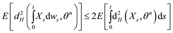
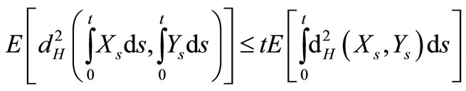
Using the properties of the Hausdorff distance one can formulate the following results
Lemma 2.1.
1) if
then 
2) if

then 
3) If  and
and  reconstants, then
Corollary 2.1. (see [7]) Let set-valued stochastic processes 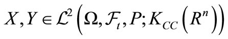 we have the following confirms:
1) ;
;
2) ;
;
3) ;
;
4) .
.
Definition 2.3. A solution  to Equation (2.2) is unique if for every
 :
:

where  is any solution to Equation (2.2).
Assume that  satisfy the following hypotheses:
(H1) For every set  the mappings
 :
:  are nonanticipating multifunctions.
(H2) There exists a constant , such that

(H3) There exists a constant , such that

(H4) There exists a function , such that

where .
.
(H5) There exists a function , such that

where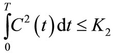 .
.
Corollary 2.2. (see [1], Theorem 7) Assume  be an
be an —measurable multifunction and F, G satisfy (H1)-(H3), then SSDE (2.2) has a unique solution and satisfies estimate
Corollary 2.3. Assume  be an
be an —measurable multifunction and F, G satisfy (H1), (H4)-(H5), then SSDE (2.2) has a unique solution and satisfies estimate

3. Main Results
In this section, we study some kinds of stability properties such as stable, asymptotically stable, exponentially stable by Lyapunov and some other stability criteria such as equi, uniform and equi-asymptotical stabilities for SSDE.
Definition 3.1. The trivial stochastic set solution of SSDE Equation (2.2) is said to be
(LS) Lyapunov stable, if for each  and
and 
there exist a , such that
implies .
.
(ALS) Asymptotical Lyapunov stable, if it is (LS) and
 .
.
(ELS) Exponent Lyapunov stable, if there exist  , such that:

Definition 3.2. The trivial stochastic set solution of SSDE Equation (2.2) is said to be:
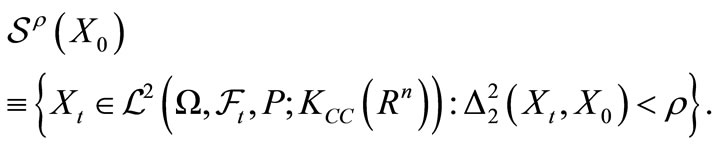
(S1) Equi-stable, if for each , and
, and  there exists
  such that
  implies that
 ,
, ;
;
(S2) Uniformly stable, if  in (S1) is independent of
 ;
;
(S3) Quasi-equi-asymptotically stable, if for each , there exists
  and
and 
such that  implies
 , for all
 ;
;
(S4) Quasi-uniformly-asymptotically stable, if  and
and  in (S3) are independent of
 ;
;
(S5) Equi-asymptotically stable, if (S1) and (S3) hold simultaneously;
(S6) Uniformly asymptotically stable, if (S2) and (S4) hold simultaneously;
(S7) Exponent-asymptotically stable, if exist  such that
  for all
Lemma 3.1. According to the Definitions 3.1 and Definition 3.2, we can say that 1) The stochastic set solution of SSDE E (2.2) is (S1) if and only if it is (LS) that means (S1)  (LS).
(LS).
2) (S6)  (ALS).
3) (S7)  (ELS).
4) (S6) or (ALS)  (S6).
(S6).
5) (S6)  (S4).
(S4).
Thus we have to prove (S1), (S6) and (S7).
Next, we present some results about (S1)-(S6) of solution with using the Lyapunov-like functions.
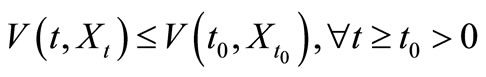
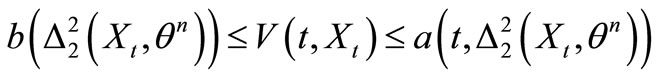
Theorem 3.1. Suppose that the positive Lyapunov-like function satisfies the following conditions:
1)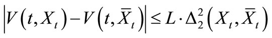 where
where  is Lipschitz constant, for all
 ,
,
 ,
, ;
;
2) The Dini derivative
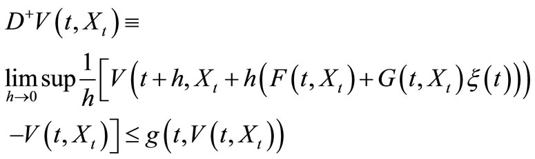
where ,
, ;
;
If  is any solution of SSDE Equation
(2.2) Such that , then we have
where  is a maximal solution of ordinary differential equation (ODE)
 (3.1)
(3.1)
Proof. Let  be any solution of SSDE Equation (2.2) existing on
 . We define the function
  so that
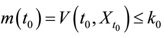 .
.
Now for small , by our assumption it follows that
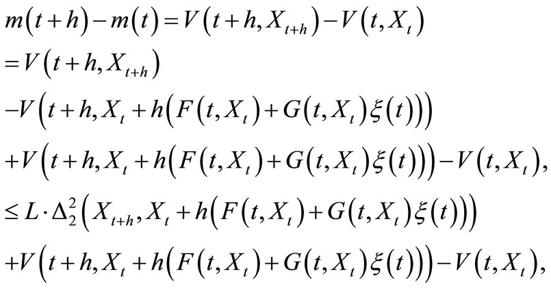
by using the Lipschitz condition give (1). Thus

Since
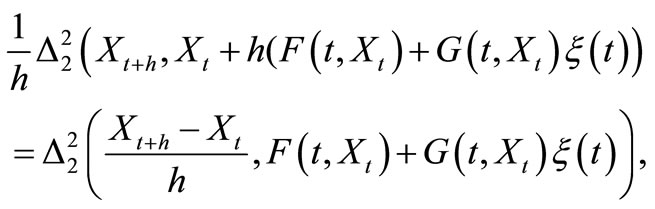
and  is any solution of SSDE Equation (2.1), we find that

We therefore have the scalar differential inequality 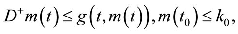 which yields, as before, the estimate
 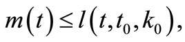 where
where  is a maximal solution of ODE (3.1). This proof is complete.
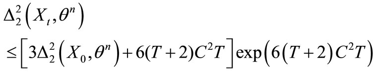
Corollary 3.1. If the Lyapunov-like function 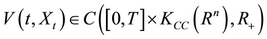 satisfies conditions in Theorem 3.1 then we have the estimate:
Next, putting
Theorem 3.2. Assume that for SSDE Equation (2.2) exists the Lyapunov like function  which satisfies the conditions of Theorem 3.1.
a) If there exist the positive functions  are strictly increasing such that:
1) 

and , then (S1) holds.
Futhermore, there exists  such that
2) If , then (S3) holds.
3) If , then (S5) holds.
b) If there exist the positive functions  are strictly increasing and
  such that:
1) 

and , then (S2) holds.
Futhermore, there exists  such that.
2) If , then (S4) holds.
3) If  then (S6) holds.
Proof. Let  and
and  be given, choosing
  such that
  with this we have (S1).
If this is not true, there would exists a stochastic set solution  of SSDE Equation (2.2) and
  such that
with . By using Corollary 3.1 and a/1, we have
 and condition
 as result, yield:
This contradiction proves that (S1) holds.
Next, we have to prove that:  there exists a
  and number
  such that:
 implies
 for
for
 . Let
. Let  and
and .
.
Choosing  such that
  with this we have (S3). If this is not true, there would exists a stochastic set solution
  of SSDE Equation
(2.2) such that,  and
and where
where , for
, for 
By using assumption (a/2) of this theorem shows that ,
,  and yields:

This contradiction proves that (S3) holds.
The affirmation for (S5) is proved analogous to the proof of the affirmations for (S1), (S3).
Next, we have to prove that (S2) holds:
By  implies
and ,
, .
.
Thus for all  and
and  the affirmation for (S1) holds, that means the affirmation for (S2) holds.
Next, we have to prove that (S4) holds. According to assumption b) of Theorem 3.2
1) 
2) 
For all , we have
As a result,

and (S4) holds.
The affirmation for (S6) is proved analogous to the proof of the affirmations for (S2), (S4).
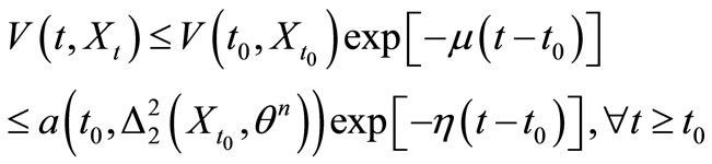
Corollary 3.2. Assume that for SSDE Equation (2.2) exists the Lyapunov like function  which satisfies the conditions of Theorem 3.1, and exist the positive numbers
  such that
 .
.
If , then (S7) holds.
Proof. The proof for (S7) is proved analogous to the proof of the affirmations for (S4).
4. Some Applications of Stochastic Set Differential Equations
For example, in a finance market we consider some stock price at time  denoted by
  which is a random variable defined on the probability space
 . Owing to the quick fluctuation of the stock price from time to time or to the existence of missing data, we may not precisely know the price
 . A possible model for this situation would be to give the upper and the lower prices (i.e. a margin for the error in the observation). Then we obtain an nterval
 , which is a special kind of a set-valued random variable, ontains not only randomness but also impreciseness, and we assume
  is certainly in this interval.
For example different, in environmental of the insurance premium, the risks is considered a main material of this industry. Beside that, the risks are random factors and associating with premiums, so insurance premiums should be built on the basis of risks to price insurance which could compensate and balance the damage occurs to their business costs. Otherwise, the risks are some kinds different and levels of influence are different, so they could influence to levels of price of the insurance premium.
Hence, we may not precisely know the price of the insurance premium such that be beneficial to company of the insurance and customers. Then, in special the case we assume  is certainly in this interval which admissible prices.
Example 4.1. (Stock prices) Let  denote the price of a stock at time
 , where
  (i.e. interval-valued). We can model the evolution of
  and the relative change of price, evolves according to the SSDE under the form
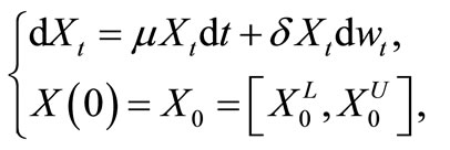 (4.1)
(4.1)
for all , for certain constants
 , called the drift and the volatility of the stock.
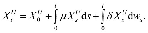
Since coefficients in Equation (4.1) satisfy the conditions in Corollary 2.2, there is a unique solution of Equation (4.1). This means that for  SSDE (4.1) satisfies the following interval-valued stochastic differential equation
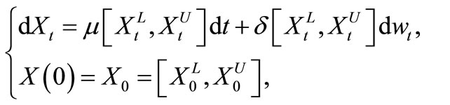 (4.2)
(4.2)
for all . That is,
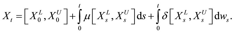
Since ,
,  and
and  are the solutions of the following stochastic differential system
 (4.3)
(4.3)
 (4.4)
(4.4)
We can slove Equation (4.3) and Equation (4.4) by classic methods. Thus, the solutions of Equation (4.3) and Equation (4.4) respecttively are
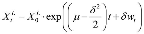
and
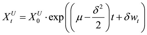 .
.
Its graphical representation can be seen in Figure 1.
From here it is easily verifiable stability criteria of solution to Equation (4.1).
5. Further Research
In the future, we will concentrate all our efforts on other properties of this kind of equation discussed in our paper, such as on the existence of extremal solutions for SSDEs (2.2). Beside that, set-valued stochastic differential equations and their solutions seem to be a starting point for
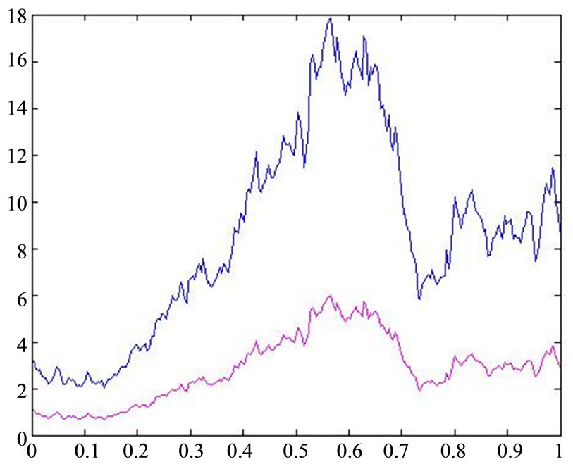
Figure 1. Solution of Example 4.1 in case μ = 2, δ = 1.
further development in the theory of control for SSDEs. Below we present the main idea, we consider the setvalued stochastic control differential equations (SSCDEs) under the form
 (4.5)
(4.5)

where 
are continuous multifunctions, state set  and
and  is different controls, inclusion: admissible control, feedback control and contraction control. The problems of the existence and properties of solutions to SSCDEs Equation (4.5) is still open.
6. Acknowledgements
The authors gratefully acknowledge the referees for their careful reading and many valuable remarks which improved the presentation of the paper. The authors thank the partial financial support of AM editorial office.
REFERENCES
- M. T. Malinowski and M. Michta, “Stochastic Set Differential Equations,” Nonlinear Analysis: Theory, Methods & Applications, Vol. 72, No. 3-4, 2010, pp. 1247-1256. doi:10.1016/j.na.2009.08.015
- F. Hiai and H. Umegaki, “Integrals, Conditional Expectations and Martingales for Multivalued Functions,” Journal of Multivariate Analysis, Vol. 7, No. 1, 1977, pp. 147- 182.
- J. P. Aubin and G. Da Prato, “The Viability Theorem for Stochastic Differential Inclusion,” Stochastic Analysis and Applications, Vol. 15, No. 5, 1997, pp. 783-800.
- J. Motyl, “Stochastic Functional Inclusion Driven by Semimartingle,” Stochastic Analysis and Applications, Vol. 16, No. 3, 1998, pp. 517-532. doi:10.1080/07362999808809546
- M. T. Malinowski and M. Michta, “Stochastic Fuzzy Differential Equations with an Application,” Kybernetika, Vol. 47, No. 1, 2011, pp. 123-143.
- M. Michta, “On Set-Valued Stochastic Integrals and Fuzzy Stochastic Equations,” Fuzzy Set and Systems, Vol. 177, No. 1, 2011, pp. 1-19.
- E. J. Jung and J. H. Kim, “On Set-Valued Stochastic Integrals,” Stochastic Analysis and Applications, Vol. 21, No. 2, 2003, pp. 401-418. doi:10.1081/SAP-120019292
- J. Zhang, “Set-Valued Stochastic Integrals with Respect to a Real Valued Martingales,” In: D. Dubois, M. A. Lubiano, H. Prade, et al., Eds., Soft Method for Handling Variability and Imprecision, Springer, Berlin, 2008, pp. 253-259.
- J. Li and S. Li, “Set-Valued Stochastic Lebesgue Integral and Representation Theorems,” International Journal of Computational Intelligence Systems, Vol. 1, No. 2, 2008, pp. 177-187. doi:10.2991/ijcis.2008.1.2.8
- J. Zhang, S. Li, I. Mitoma and Y. Okazaki, “On Set-Valued Stochastic Integrals in an M-Type 2 Banach Space,” Journal of Mathematical Analysis and Applications, Vol. 350, No. 1, 2009, pp. 216-233. doi:10.1016/j.jmaa.2008.09.017
- N. D. Phu, N. Van Hoa and N. M. Hai, “Some Kinds of Controls for Boundedness Properties of Stochastic Set Solutions with Selectors,” International Journal of Evolution Equations, Vol. 5, No. 4, 2011, pp. 54-69.
- N. D. Phu, N. Van Hoa and H. Vu, “On the Stability Properties by Quasi-Expectation of Stochastic Set Solutions with Selectors,” Journal of Nonlinear Evolution Equations and Applications, Vol. 3, 2011, pp. 57-71.
- N. D. Phu, N. Van Hoa, N. M. Triet and H. Vu, “Boundedness Properties of Solutions to Stochastic Set Differential Equations with Selectors,” International Journal of Evolution Equations, Vol. 6, No. 2, 2012.
- V. Lakshmikantham, T. G. Bhaskar and D. J. Vasundhara, “Theory of Set Differential Equations in Metric Spaces,” Cambridge Scientific Publisher, Cambridge, 2006.