Modern Economy
Vol.5 No.1(2014), Article ID:42332,7 pages DOI:10.4236/me.2014.51010
Making Every Dollar Count: Local Government Expenditures and Welfare
1Department of Agricultural Economics, Kansas State University, Manhattan, USA
2Department of Agricultural Economics, Indiana University of Pennsylvania, Indiana, USA
Email: pgaray@agecon.ksu.edu, yacobaz@ksu.edu, Alexi.Thompson@iup.edu
Copyright © 2014 Pedro V. Garay et al. This is an open access article distributed under the Creative Commons Attribution License, which permits unrestricted use, distribution, and reproduction in any medium, provided the original work is properly cited. In accordance of the Creative Commons Attribution License all Copyrights © 2014 are reserved for SCIRP and the owner of the intellectual property Pedro V. Garay et al. All Copyright © 2014 are guarded by law and by SCIRP as a guardian.
Received October 17, 2013; revised November 17, 2013; accepted November 24, 2013
KEYWORDS
Local Government; Expenditure; Well-Being
ABSTRACT
The paper aims at examining the relationship between the allocations of funds at the local government level and the economic well-being of citizens. The results of this study help shed light on ways to get the best out of every dollar spent by local governments. Three empirical proxy measures for citizen well-being were used in the estimation of three different panel data models. Results suggest that some types of government expenditure can have a positive influence on citizen well-being. The analysis provides insights into how economic development policies may be conceived by local governments to ensure sustained economic prosperity of its citizens.
1. Introduction
Government spending and taxation can have significant effects on the economy and on the lives of individuals. Government carries out a number of important economic functions including correcting inefficiencies in the allocation of goods and services by levying taxes or providing subsidies to correct externalities. Governments also provide public goods such as national defense, police protection, and infrastructure. Governments can also have an economic stabilizing function to reduce unemployment or inflation [1].
Many politicians advocate increases in government spending, particularly during recessions, to stimulate economic growth. Other politicians oppose increases in government spending as it contributes to the government deficit in the long run. Empirical evidence is mixed; studies suggest that some types of public social welfare expenditures can improve economic well-being. Hungerford [1] finds that countries with higher public social welfare expenditures relative to GDP have lower relative poverty rates. Gupta, Verhoeven, and Tiongson [2] use cross-country data for 44 countries to assess the relationship between public spending on health care and the health status of poor. Their results suggest that increased public spending on health alone will not be sufficient to significantly improve health status. Kenworthy [3] studies the effects of social welfare policy extensiveness on poverty rates across fifteen industrialized nations over the period 1960- 91 using both absolute and relative measures of poverty. The results strongly support the conventional view that social-welfare programs reduce poverty. Fan, Hazell and Thorat [4] develop a simultaneous equation model using state-level data for 1970-1993 to estimate the direct and indirect effect of different types of government expenditure on rural poverty and productivity growth in India. They find that investment in rural road, agricultural research and education reduces poverty, but health has only a modest impact on growth and poverty.
This paper examines the consequences of local government spending, especially public social welfare expenditures, on the well-being of the citizens in the US. Local government is defined to encompass counties, municipalities, towns and townships as well as special purpose governments such as water, fire and library district governments and independent school district governments. Using US Census Bureau’s Census of Governments data [5], it was found that there were a total of 39,044 counties and sub-county governments in the United States and 50,432 special purpose governments, giving a total of 89,476. This gives a framework of the number of government entities under consideration in the rest of the paper. However, for the purposes of this paper, the local governments have been aggregated within states and assessed over time, from 1990 to 2005.
2. Measures of Citizens’ Well-Being
Three empirical proxy measures of citizens’ well-being are used in this paper including poverty rate, median income, and disposable income. These measures are typical in similar studies [6-8]. The poverty rate within a region (e.g., state, county, and municipality) is a common measure used to define citizen well-being. To determine if a family is living in poverty, the US Census Bureau compares a family’s total income against a set of money income thresholds which vary by family size and composition. These thresholds are based on the ones designed by Mollie Orshansky in the 1960’s. If the total income is less than the appropriate threshold, then the family and all of the individuals within the family are considered to be in poverty. Although the money income thresholds do not vary across the nation, they are modified each year to account for inflation using the Consumer Price Index for All Urban Consumers (CPI-U) [9].
In the US, money income, market income, post-social insurance income and disposable income are four measures of income that can be used to estimate economic well-being and the impact of taxes and governmental transfers. Money income is used in the official definition of poverty and the other income measures differ from each other based on the inclusion or exclusion of certain monetary components. As a result, income distribution changes depending on the income measure used [10].
Money income includes all money income earned or received by individuals who are 15 years or older before tax deductions or other expenses. This measure does not include capital gains, lump-sum payments or non-cash benefits (e.g., payments from insurance companies, worker’s compensation or pension plans). Market income consists of all resources available to families based on market activities. It is similar to money income but government cash transfers and imputed work expenses excluding work expenses are deducted. However, imputed net realized capital gains and imputed rental income are included in this definition. This measure can be used as a reference point when investigating the effect of government activity on income and poverty estimates [10].
Post-social insurance income consists of governmental programs that affect everyone and not those solely created for people with low income. This measure is similar to market income except that non-means-tested government transfers are included (e.g., social security, unemployment compensation and worker’s compensation). Therefore, households who receive income from at least one of the non-mean-tested government transfers have a higher median income under post-social insurance income measure than market income [10].
The final income measure is disposable income, which represents the net income households have available to meet living expenses. According to Smeeding and Sandstorm [7], the best income definition when determining poverty and poverty rates is disposable cash or near-cash income. This measure includes money income, imputed net realized capital gains, imputed rental income and the value of noncash transfers (e.g., food stamps, subsidized housing and school lunch programs). Excluded from this measure are imputed work expenses, federal payroll taxes, federal and state income taxes and property taxes for owner-occupied homes. Of the four income measures, disposable income has the lowest median income. A comparison between post-social insurance income and disposable incomes highlights the net impact of meanstested government transfers and taxes. By comparing market income and disposable income, the net impact of government transfers and taxes on income and poverty estimates can be determined [10].
The National Academy of Sciences (NAS) advocates for a revision of the methods used by the US Census Bureau to measure poverty. One criticism of the official poverty definition is that pre-tax income (i.e., money income measure) is used to determine who is in poverty. Therefore, the effect of how taxes, non cash benefits and work-related and medical expenses on people’s wellbeing are not taken into account. Additionally, the effect of policy changes on people who are considered to be in poverty cannot be observed. Another criticism is that the official poverty definition does not reflect variation in costs across the nation. NAS believes that the official thresholds do not accurately represent the increase in expenses or the economies of scales which occur with increases in the family size [9].
This criticism surrounding how poverty rates are calculated in the US provides the rationale for examining alternative measures of citizen well-being in addition to using poverty rate. That is, we will investigate how local government expenditure affects three different measures of citizen well-being; poverty rate, median income and disposable income.
The foregoing discussion focuses on objective metrics of well-being. However, there is increasing consensus among sociologists and economists that well-being of individuals cannot be described solely by objective social situation alone [11]. Thus, there are calls for a more nuanced view of well-being that meshes the broader social trends that is placing higher value on the quality of life rather than on economic success [12] and shifts focus within the social sciences to recognize the limits of revealed preferences, upon which most of consumer economics rests. The foregoing have caused the adoption of subjective well-being from its psychology domain and incorporated it into economics and sociology in attempts to understand how individuals within a community assess their well-being. While this paper makes no attempt to incorporate these broader and richer measures of individual subjective measures of well-being, it is discussed here to anchor our observations about the limitations of a macro-level analysis such as this as we search for the influence of local government expenditure on citizen wellbeing and local economic development.
3. Data
An unbalanced panel data collected from the US Census Bureau’s annual survey of local government finances as well as state population sizes from 1991 to 2005 for fifty states plus the District of Columbia was used. However, local government finances data for the years 2000 and 2002 were not available and so these data points were treated as missing points. The expenditure categories include education, health, transportation, public safety, environment and housing, and government administration. The well-being measures (poverty rate, median income, and disposable income) were collected directly from US Census Bureau annual data for these communities. The absolute magnitude of local government expenditures varied significantly from state to state as so did the population sizes of the states. In order to avoid scaling problems associated with different expenditure and population sizes of the respective local governments, the expenditure categories were expressed in per capita terms. To do this, the local government expenditures in each state were divided by the population size of each state. The population data for the respective states were obtained from the Census Bureau database. Similarly, the poverty rate was expressed in percentage terms and both the median income and the disposable income for each state were also expressed as a proportion of the average values for the United States All variables are expressed in natural logarithms.
4. Government Spending Measures
Education spending includes spending on colleges and other institutions but does not include agricultural extension services. Spending on health includes immunization clinics, research and education, and public health administration. Public safety spending includes police and fire protection. Transportation includes spending on highways and air transportation. Environment and housing includes spending on parks and recreation and solid waste management. Government administration includes spending on planning and zoning. For a complete definition of the spending categories, please see the US Census Bureau. All expenditure categories are assumed to have a positive effect on economic well-being.
5. Methods
Following the work of Wald [13], Hildreth and Houck [14], and Swamy [15,16], we use three panel data models to assess the relationship between the measures of wellbeing and local government expenditure, including pooled ordinary least square (POLS), fixed effects model (FE), and random effects model (RE). The pooled ordinary least square model is used assuming that there is no individual heterogeneity between the states. However, the fixed effects and the random effects models account for heterogeneity among the states as will be explained further under each model. The study followed series of tests to choose appropriate models as shown in the results section.
Under the pooled-OLS model, we have
 (1)
(1)
where  is the dependent variable (poverty rate, median income, disposable income) of the ith state at time t,
  represents the independent variables, βs are the estimated coefficients, α represent the intercept and uit is the unobserved error term. The POLS model increases the probability of a bias occurring due to unobserved heterogeneity (uit and
  may be correlated). If it is believed that the error terms and the independent variables are not correlated, then using POLS can give unbiased estimates. Otherwise the bias can be addressed by decomposing the error term in two components:
 (2)
(2)
where 𝜇i is a state-specific error and  represents an idiosyncratic error.
Since the state-specific error does not vary over time, every state has a fixed value on this latent variable. Unlike the state-specific error, the idiosyncratic error,  , varies over states and time and it should satisfy the assumptions for the standard OLS error terms.
In the Fixed Effect (FE) estimation, after some manipulations we can get
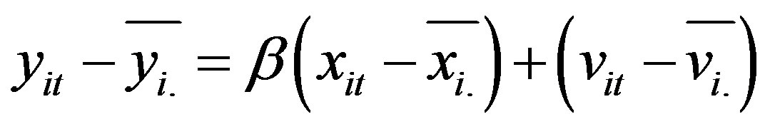 (3)
(3)
which can be estimated by POLS or FE estimator. Timeconstant unobserved heterogeneity is not a problem allowing the FE-estimator to be successful in identifying the true causal effect. In the Random Effects (RE) estimation, we assume that the 𝜇i’s are random (independent and identically distributed random-effects) and that Cov (Xit,i) = 0.
We run a set of regressions using each of the above models. The regressions use expenditures in education, health, transportation, public safety, environment and housing, and government administration as the explanatory variables. The dependent variables are poverty rate, median income, and disposable income.
6. Results
Results from the POLS model, Fixed Effects (FE) model and the Random Effects (RE) model are displayed in Table 1. Each model was analyzed with each measure of economic well-being.
Fixed effects are tested by the (incremental) F test, while random effects are examined by the Lagrange
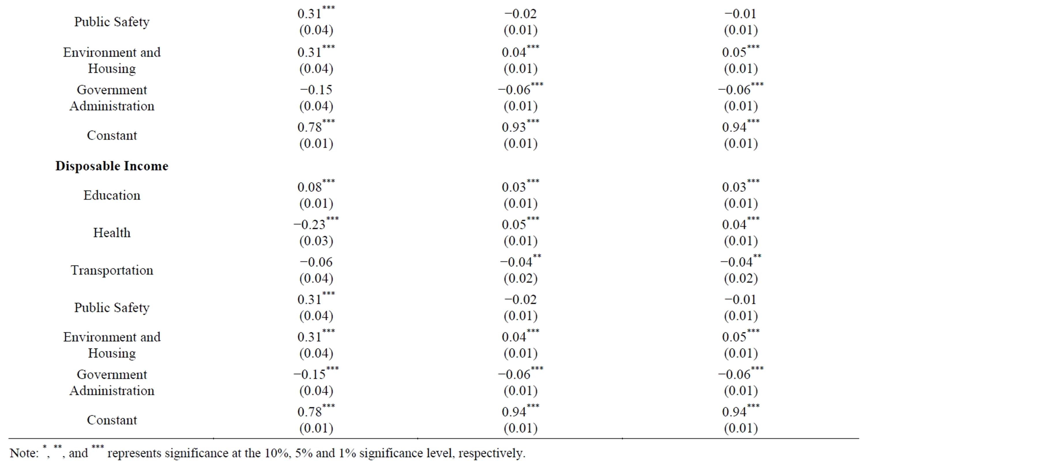
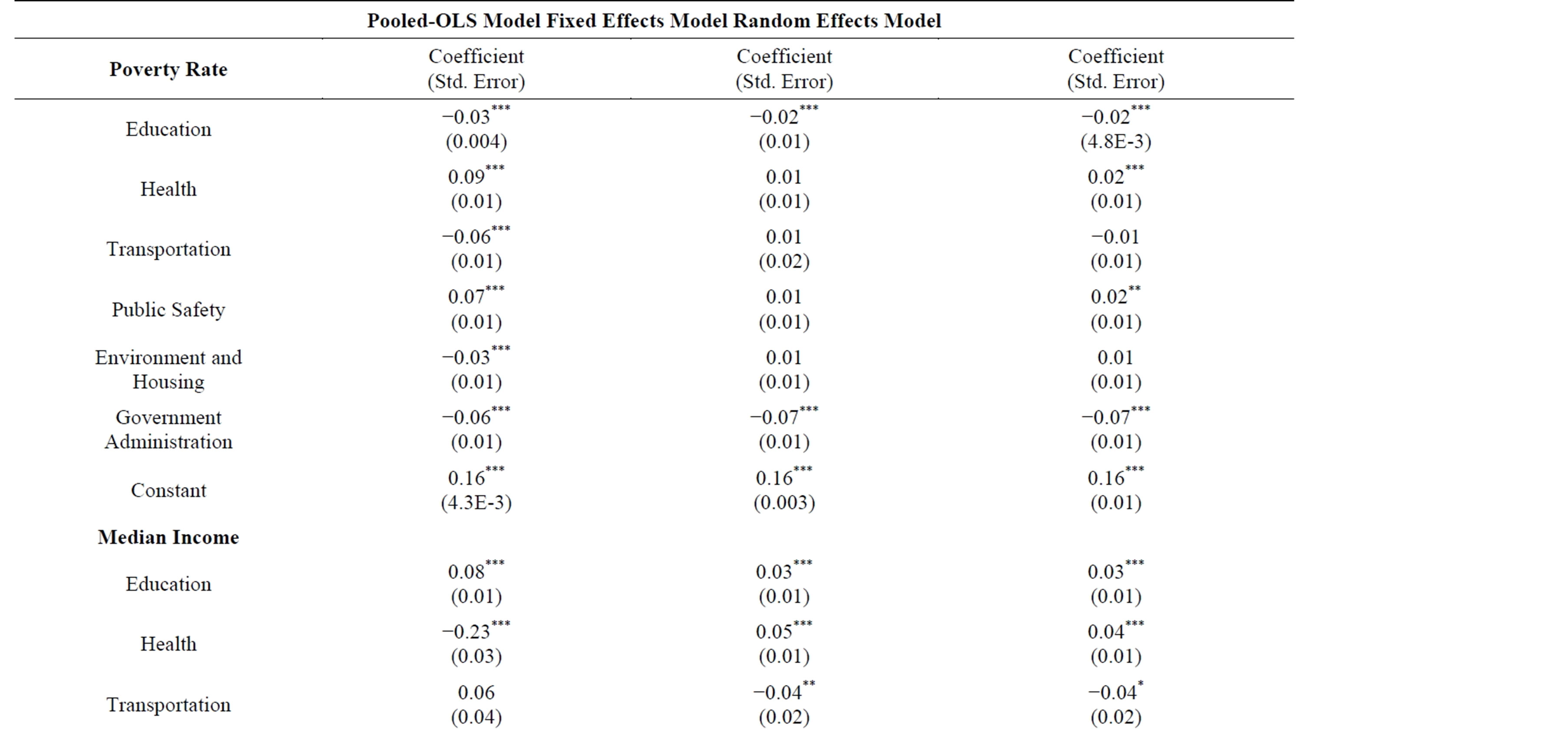
Table 1. Regression results from Pooled-OLS model, fixed effects model and random effects model.
Multiplier (LM) test [17]. If the null hypothesis (of the F test or LM test) is not rejected, the POLS regression is favored over FE or RE models, respectively. When poverty rate and disposable income are dependent variables, results of the F test and LM test indicate FE and RE models are preferred to POLS estimation. However, when median income was used as a dependent variable the test failed to reject the null hypotheses, implying that for this model the POLS model is preferred to both the FE and RE models.
When either FE and RE models are preferred to the POLS model, the Hausman specification test [18] was applied to compare the FE and RE models. The Hausman specification test compares FE versus RE under the null hypothesis that the individual effects are uncorrelated with the other regressors in the model [18]. If correlated (H0 is rejected), a random effect model produces biased estimators, violating one of the Gauss-Markov assumptions; so a FE model is preferred. Examining whether the dependent variable (i.e., poverty rate, median income, disposable income) is location dependent is crucial to identify the true causal effect. The FE model controls state heterogeneity, which is supposed to be time constant, and helps identify the relationship between the dependent variables and explanatory variables. When the poverty rate and disposable income were used as dependent variables, we used the Hausman homogeneity test to determine if there was a systematic difference in coefficients between the FE and the RE models. Results indicate that there is a significant difference between the two models suggesting that there is certain covariance present between 𝜇i’s and Xit’s implying FE is preferred to RE.
Some of the results, especially the signs on the coefficients, were not consistent in the different models. For example, in the upper panel of Table 2, the signs for the transportation variable were positive for the POLS and RE models, but negative sign for the FE model. So, for the foregoing discussions, we have used variables that were consistent in all the models.
When poverty rate is used as a dependent variable, the
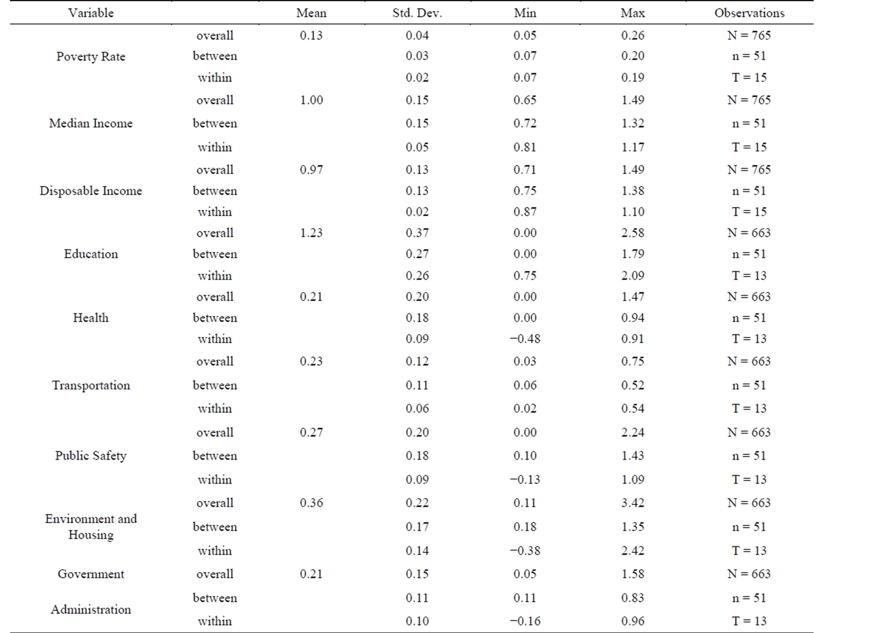
Table 2. Descriptive statistics of the variables used in the study.
estimated coefficients for education, government administration expenditures, and public safety were statistically significant. According to this model, expenditures on both education and government administration would reduce the poverty rate. For example, a one percent increase of expenditure by local government on education would cause poverty rate in the United States to decrease by 0.03%. A 1% increase in government administration expenditures reduces poverty rate by 0.06%.
In the POLS model where the median income is used as the dependent variable, most of the variables are statistically significant. Public safety and government administration are not significant. Using the POLS model to predict the effects of government expenditure measures on median income, a 1% increase in expenditure on education would cause median income to increase by 0.08%. Expenditures on environment and housing (e.g. parks and recreation, and housing and community development) and public safety cause the largest increase in median income as a proportion of average US median income compared to other expenditure categories.
Using the FE model, when we analyze the relationship between the local government expenditure and the disposable income, expenditures on education and environment and housing have positive effect on disposable income. Government administration expenditures negatively affect disposable income. Using the fixed effects model to predict the disposable income, a 1% increase in expenditure on education would cause disposable income to increase by 0.03%.
7. Conclusions
In this study, we focused on the relationship between local government expenditure and citizen well-being. We hypothesized that the allocation of local government expenditure influenced the wealth status of its citizens. Three panel data models (pooled-OLS, FE model and RE model), each with three different dependent variables (poverty rate, median income and disposable income) were estimated to determine the impact of government expenditure on citizen well-being. Most of the variables in the regressions are statistically significant implying that government expenditures do affect citizen well being. The signs for education variable coefficients unambiguously matched expectations. Expenditure in education has a statistically significant impact on well-being regardless of the model.
Depending on the objectives of the local government, policy instruments can be designed to target specific citizen well-being measures. For example, based on the results of the current study, if the priority of the local governments is to reduce poverty level, more per capita expenditure may be allocated on government administration. If local government wants to target median income, the results would suggest more expenditure on environment and housing (e.g. parks and recreation, and housing and community development) which cause the largest increase in median income as a proportion of average US median income compared to other expenditure categories.
REFERENCES
- T. L. Hungerford, “The Effects of Government Expenditures and Revenues on the Economy and Economic WellBeing: A Cross-National Analysis,” CRS Report for Congress, 2006.
- S. Gupta, M. Verhoeven and E. R. Tiongson, “Public Spending on Health Care and the Poor,” Health Economic, Vol. 12, No. 8, 2003, pp. 685-696. http://dx.doi.org/10.1002/hec.759
- L. Kenworthy, “Do Social-Welfare Policies Reduce Poverty? A Cross-National Assessment,” Social Forces, Vol. 77, No. 3, 1999, pp. 1119-1139.
- S. Fan, P. Hazell and S. Thorat, “Government Spending, Growth and Poverty in Rural India,” American Journal of Agricultural Economic, Vol. 82, No. 4, 2000, pp. 1038- 1051. http://dx.doi.org/10.1111/0002-9092.00101
- Federal, State, and Local Governments, “State and Local Government Finances,” US Commerce Department, Washington DC, 2007. http://www.census.gov/govs/www/index.html
- T. M. Smeeding and D. H. Sullivan, “Generations and the Distribution of Economic Well-Being: A Cross-National View,” The American Economic Review, Vol. 88, No. 2, 1998, pp. 254-258.
- T. M. Smeeding and S. Sandstörm, “Poverty and Income Maintenance in Old Age: A Cross-National View of LowIncome Older Women,” Feminist Economics, Vol. 11, No. 2, 2005, pp. 163-174.
- J. D. Smith and J. N. Morgan, “Variability of Economic Well-Being and Its Determinants,” American Economic Review, Vol. 60, No. 2, 1970, pp. 286-295.
- B. D. Proctor and J. Dalaker, “Poverty in the United States: 2002,” US Census Bureau, Washington DC, 2003.
- United States Census Bureau (US Census Bureau), “The Effect of Taxes and Transfers on Income and Poverty in the United States: 2005,” US Department of Commerce, Washington DC, 2007.
- R. A. Easterlin, “Happiness in Economics,” Edward Elgar, Cheltenham, 2002.
- R. Inglehart, “Cultural Shift in Advanced Industrial Society,” Princeton University Press, Princeton, 1990.
- A. Wald, “A Note on Regression Analysis,” Annals of Mathematical Statistics, Vol. 18, No. 4, 1947, pp. 586-589. http://dx.doi.org/10.1214/aoms/1177730350
- C. Hildreth and J. P. Houck, “Some Estimators for a Linear Model with Random Coefficients,” Journal of the American Statistical Association, Vol. 63, No. 322, 1968, pp. 584-595. http://dx.doi.org/10.2307/2284029
- P. A. V. B. Swamy, “Statistical Inference in Random Coefficient Regression Models and Its Applications in Economics,” Annals of Mathematical Statistics, Vol. 38, No. 2, 1967, pp. 1941-1947.
- P. A. V. B. Swamy, “Efficient Inference in a Random Coefficient Regression Model,” Econometrica, Vol. 38, No. 2, 1970, pp. 311-323. http://dx.doi.org/10.2307/1913012
- T. S. Breusch and A. R. Pagan, “The Lagrange Multiplier Test and Its Applications to Model Specification in Econometrics,” Review of Economic Studies, Vol. 47, No. 1, 1980, pp. 239-253. http://dx.doi.org/10.2307/2297111
- J. A. Hausman, “Specification Tests in Econometrics,” Econometrica, Vol. 46, No. 6, 1978, pp. 1251-1271. http://dx.doi.org/10.2307/1913827