Wireless Engineering and Technology
Vol.2 No.3(2011), Article ID:5830,12 pages DOI:10.4236/wet.2011.23026
Optimal Territorial Resources Placement for Multipurpose Wireless Services Using Genetic Algorithms
![]()
1Department of Applied Electronics, Rome 3 University, Rome, Italy; 2Department of Information, Electronics and Telecommunication Engineering SAPIENZA—University of Rome, Rome, Italy.
Email: fabio.garzia@uniroma1.it
Received February 8th, 2011; revised March 20th, 2011; accepted April 5th, 2011.
Keywords: Genetic Algorithm, Wireless Optimization, Digital Terrain Elevation Data (Dted), Wireless Resources Placement
ABSTRACT
This paper presents a study for finding a solution to the placement of territorial resources for multipurpose wireless services considering also the restrictions imposed by the orography of the territory itself. To solve this problem genetic algorithms are used to identify sites where to place the resources for the optimal coverage of a given area. The used algorithm has demonstrated to be able to find optimal solutions in a variety of considered situations.
1. Introduction
In a lot of enforced contexts there is the need to place some resources to guarantee the best coverage of an assigned region. It’s sufficient to consider the wide-spread use of means of communication that exploit the air as a transfer channel like television and cellular services or to consider the need to watch over a region where some sensors are used to guarantee the safety from different threats like the terrorism [1-3].
For this reason every day it is necessary to find new places to install systems of transmission and/or reception like antennas, base stations for cellular phones and sensors.
Actually this kind of operation is not automatic and it is made through the experience of people that place resources by analysing the map of the interested region. Naturally this process is approached by the iterative computation of the effective obtained coverage for any attempt.
The purpose of this paper is to describe a new technique to automatize the initial phase of this process by elaborating an algorithm for the placement of resources on the ground to guarantee the best coverage of a given region. In this context the term “best” must be considered in a wider sense because it’s simplified by thinking about the wide coverage as the only requirement of the problem. The problem instead is more complex: the term “best” is referred to a coverage obtained by the balancing of different parameters required by the problem. Our purpose is to obtain a wide coverage under the condition that the number of placed resources is the minimum possible and that they work over a certain percentage of their coverage capability. This implies that the resources that don’t give a significant contribution to the coverage because of the presence of obstacles or because of superposition must be eliminated from the solution grid causing the reduction (even if it is neglect able) of the percentage of the obtained coverage. This let understand why the reaching of integral coverage of the considered territory is really impossible. Naturally these are only some of the conditions that can be imposed to the algorithm. In general it’s possible to use different kind of resources, to have a nonuniform coverage like in urban environment, to consider the coverage of the sensors in 2 or 3 dimensions, to have resources already placed [4,5] on the ground. All these conditions make the problem represented by a multiobjective and non-linear function so it’s quite difficult to find an optimal solution. In the solution of the problem it’s also necessary to take care of the orography of the ground using Digital Terrain Elevation Data with discrete resolution (DTED) as we made in the present work, to face real situations.
The problem is quite complex both from a theoretical (a closed analytical solution doesn’t exist and it’s necessary to proceed with subsequent approximations) and from a computational point of view (it’s necessary to reduce computation time to reasonable values) [6-38].
To solve the considered problem, different algorithms have been analysed. These algorithms, besides the problem’s characteristics, have been evaluated by other typical characteristics or by their own implementation. Because of the problem’s complexity, it’s assumed that the algorithm works by subsequent iterations, reaching cycle after cycle the better solution, but not necessary the optimal solution; this kind of behaviour, coherent for a planning algorithm, allows the final user to get early a solution and to be able to decide if and how long to wait for a better solution. The purpose of this paper is to find an algorithm characterized by a certain number of useful properties that are:
1) To provide quickly a solution: an algorithm that provides a solution from the first iterations is preferred to one that needs more iterations;
2) To provide iteration after iteration better solutions: the algorithm have to provide gradually better solutions increasing the number of iterations. The solution’s goodness depends on the elaboration time too. If the solution isn’t satisfying, the algorithm must be able to continue with the research starting from the last found solution;
3) To reach the optimal solution: is the capability of the algorithm to reach the optimal final solution;
4) To provide the distance from the optimal solution: in the solution of practical problems, the knowledge of the distance from the optimal solution is maybe more important than the reaching of solution itself; in fact the knowledge of the distance between the actual solution and the optimal one allows to evaluate if and when it is opportune stopping the research for a better solution;
5) To reduce computational load: it’s important to find an algorithm that uses the minimum number of operations to reduce resources and computational time.
This research leads to analyse different kinds of algorithms that have already been used to solve similar problems or that can be adapted to the solution of this problem. For example algorithms of linear planning and evolutionary algorithms have been analyzed. Genetic Algorithms, that are evolutionary algorithm based on the concepts of Selection, Crossover [6-10] and Mutation [15], have demonstrated to be the best one.
This paper is structured as follows. In Section 1 the model used for sensors and the study of the objective function is presented. In Section 1 the coverage algorithm is presented. In Section 3 the genetic algorithm used to solve the problem is described. In Section 4 the fitness function of genetic algorithm is formulated. In Section 5 the computational complexity and convergence time is discussed. Section 6 presents the experimental results. Finally, Section 7 discusses some conclusions and considers possible future developments.
2. Coverage Algorithm
To verify the goodness of a solution it is necessary to evaluate the coverage obtained by the placement of the resources of the solution itself so it has been necessary to create a linear algorithm that evaluates the coverage of a single resource.
The main idea is that the Genetic Algorithm places resources on the ground, cycle by cycle. For every placed resource a circular coverage area characterized by a ray R is considered. To evaluate the effective territorial coverage of every resource a coverage algorithm that works using the point of placement of the resource itself and the related DTED data is used.
In Figure 1 a scheme of the working parameters of the mentioned algorithm is shown:
In the Figure 1 we have the following quantities:
• j = point where the resource is placed;
• j + 1 = cell near the one where the resource is placed;
• h(j + 1) = altitude in the cell j + 1;
• heq(j + 2) = equivalent altitude in the cell j + 2;
• P = quantity to add to h(j + 1) to obtain heq(j + 2);
• h(j + 2) = altitude in the cell j + 2;
• hvis = visibility altitude that is the altitude we consider for the visibility of the cells.
Starting from the point where the resource is placed, for every cell of the grid that the considered resource potentially covers, the equivalent altitude is evaluated for the next cell using a linear equation derived from a simple ratio between triangles:
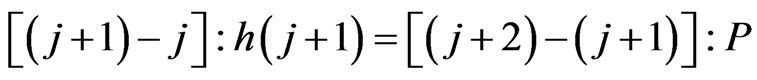 (1)
(1)
Solving Equation (1) with respect to P we have:
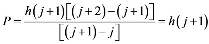 (2)
(2)
From Figure 1, using Equation (2), we have:
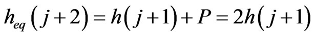 (3)
(3)
This quantity is used to verify if the cells next to the one we consider can be viewed to the visibility altitude.
The initial conditions of this algorithms are:
1) The visibility altitude is higher than the maximum of the altitude of the grid;
2) The terrestrial curvature doesn’t influence the evaluation;
3) The coverage area is reduced to a circumference
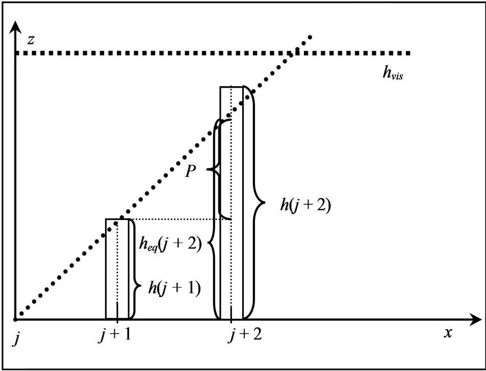
Figure 1. Context of the coverage algorithm.
characterized by a certain ray R without loss of generality since different shaped coverage diagrams with reduced increases of computation times can be also considered.
In this study we used two different resources characterized by a coverage ray R1 and R2 (R1 > R2) respectively; this allows of simplifying the algorithm without any loss of generality.
The evaluation of effective coverage is done following selected directions: the choice of these directions is explained in the following. For every direction the flow chart representing the working principle of the algorithm is shown in Figure 2.
The steps that characterize the algorithm are:
1) We start evaluating the first P that is the one between the cell in which the resource is placed and the next one. If P is smaller than zero it means that the cell next to the cell where the resource is placed has an altitude lower so it is visible at the visibility altitude. It’s necessary to evaluate P while it is negative or at a distance as long as the ray of the resource is covered. When a P greater than zero is found we evaluate the equivalent altitude and we go to the next step;
2) We compare the equivalent altitude with respect to the visibility altitude: if this quantity is smaller than the other we stop the evaluation along that ray and the evaluation goes on the next ray, otherwise we go to the next step;
3) We compare the equivalent altitude with respect to the altitude of the cell. If the equivalent altitude is greater than the altitude of the cell it is visible at the visibility altitude and the algorithm goes on with the next ray. If the visibility altitude is smaller we have to control that the altitude of the cell is smaller than the visibility altitude and if it’s true the value of P is changed with the current value and the cell is visible at the visibility altitude.
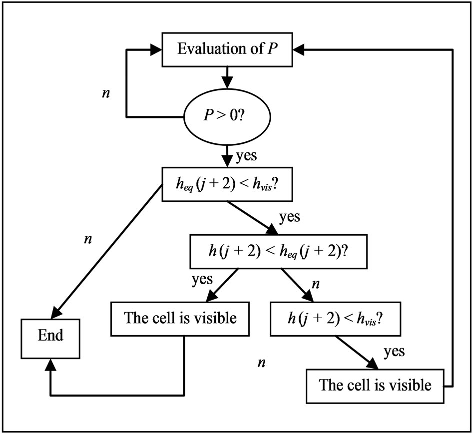
Figure 2. Scheme of the coverage algorithm.
These 3 steps are applied to the whole coverage area of the resource along the directions whose choice is explained in the following sections. For this reason it’s necessary to insert a cycle in this evaluation so that it is applied to every ray derived from the angular step chosen. Moreover it’s necessary to cover the holes between two adjacent rays.
The Figure 3 represents the way we used to reduce the coverage of a resource characterized by a coverage ray R.
The angle α is the angle formed by the ray along which we are evaluating the coverage and the x axis and it is equal to the angular step. In Figure 3 it is possible to see that the projection on the axis of the considered ray is proportional to the sine and cosine of the angular step.
The algorithm along a ray stops when the sum of the increments is greater than the projection of the point on the axis. The mentioned values are equal to R*cos α and R*sin α, as shown in Figure 4.
To cover the not analysed cells between two rays we use an algorithm very conservative that penalizes the coverage but in this way we are sure of the visibility of the cells that are not evaluated. The procedure is based on the memorization of the positions of the visible cells of the rays we took into consideration: after memorizing the positions of two adjacent rays, the cells between the two rays are considered visible. The final effect is the one shown in Figure 5. It’s evident that the more little the angular step is and the more refined the calculus of the coverage is, even if this implies an increase of computation time due to the increase of the number of operations which must be executed. A solution is represented by the use of a large angular step in the first generations, to reduce it and to refine the solution in a second time.
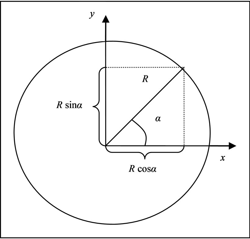
Figure 3. Scheme of resource’s coverage.
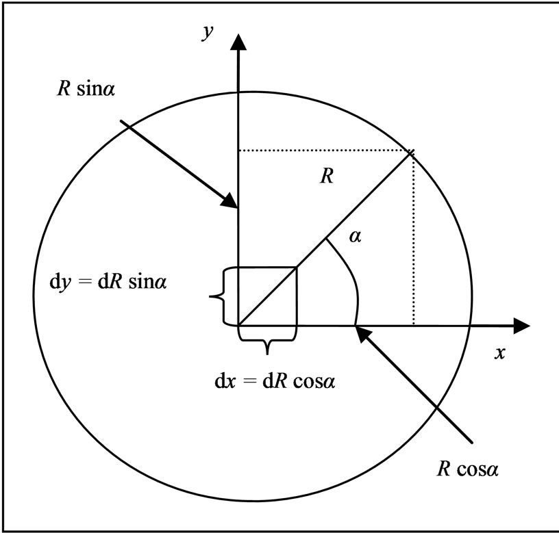
Figure 4. Increments on the rays.
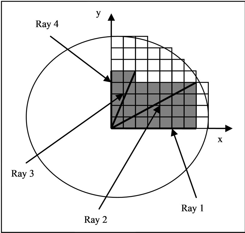
Figure 5. Coverage of the holes.
3. Spatial Resources Allocation Genetic Algorithm
Genetic algorithms are considered wide range numerical optimisation methods, which use the natural processes of evolution and genetic recombination. Thanks to their versatility, they can be used in different application fields [10-38].
The algorithms encode each parameters of the problem to be optimised into a proper sequence (where the alphabet used is generally binary) called a gene, and combine the different genes to constitute a chromosome. A proper set of chromosomes, called population, undergoes the Darwinian processes of natural selection, mating and mutation, creating new generations, until it reaches the final optimal solution under the selective pressure of the desired fitness function.
GA optimisers, therefore, operate according to the following nine points:
1) Encoding the solution parameters as genes;
2) Creation of chromosomes as strings of genes;
3) Initialisation of a starting population;
4) Evaluation and assignment of fitness values to the individuals of the population;
5) Reproduction by means of fitness-weighted selection of individuals belonging to the population;
6) Recombination to produce recombined members;
7) Mutation on the recombined members to produce the members of the next generation;
8) Evaluation and assignment of fitness values to the individuals of the next generation;
9) Convergence check.
The coding is a mapping from the parameter space to the chromosome space and it transforms the set of parameters, which is generally composed by real numbers, in a string characterized by a finite length. The parameters are coded into genes of the chromosome that allow the GA to evolve independently of the parameters themselves and therefore of the solution space.
Once created the chromosomes it is necessary to choose the number of them which composes the initial population. This number strongly influences the efficiency of the algorithm in finding the optimal solution: a high number provides a better sampling of the solution space but slows the convergence.
Fitness function, or cost function, or object function provides a measure of the goodness of a given chromosome and therefore the goodness of an individual within a population. Since the fitness function acts on the parameters themselves, it is necessary to decode the genes composing a given chromosome to calculate the fitness function of a certain individual of the population.
The reproduction takes place utilising a proper selection strategy which uses the fitness function to choose a certain number of good candidates. The individuals are assigned a space of a roulette wheel that is proportional to their fitness: the higher the fitness, the larger is the space assigned on the wheel and the higher is the probability to be selected at every wheel tournament. The tournament process is repeated until a reproduced population of N individuals is formed.
The recombination process selects at random two individuals of the reproduced population, called parents, crossing them to generate two new individuals called children. The simplest technique is represented by the single-point crossover, where, if the crossover probability overcome a fixed threshold, a random location in the parent’s chromosome is selected and the portion of the chromosome preceding the selected point is copied from parent A to child A, and from parent B to child B, while the portion of chromosome of parent A following the random selected point is placed in the corresponding positions in child B, and vice versa for the remaining portion of parent B chromosome.
If the crossover probability is below a fixed threshold, the whole chromosome of parent A is copied into child A, and the same happens for parent B and child B. The crossover is useful to rearrange genes to produce better combinations of them and therefore more fit individuals. The recombination process has shown to be very important and it has been found that it should be applied with a probability varying between 0.6 and 0.8 to obtain the best results.
The mutation is used to survey parts of the solution space that are not represented by the current population. If the mutation probability overcomes a fixed threshold, an element in the string composing the chromosome is chosen at random and it is changed from 1 to 0 or vice versa, depending of its initial value. To obtain good results, it has been shown that mutations must occur with a low probability varying between 0.01 and 0.1. The operative scheme of a GA iteration is shown in Figure 6.
The converge check can use different criteria such as the absence of further improvements, the reaching of the desired goal or the reaching of a fixed maximum number of generations.
4. Sensor Models and Object Function
4.1. Description of the Fitness Function
The solution’s scheme is shown in Figure 7.
The first step to do to solve the considered problem is to find a good coding for the sensors. In this paper sensors are modelled by four parameters: two for the position (coordinates X and Y); one for the length of the ray R of circular coverage diagram to consider two kind of different sensors; one parameter that tells us if that sensor is effectively active on the solution grid. Naturally a lot of parameters can be added to describe a sensor but this is not in the scope of the present paper that is to find a first level solution to the placement of territorial TLC resources for multipurpose services.
It’s necessary to find an objective-function that evaluates a solution’s goodness by the sensor’s model. In this case two terms are selected, the first relative to the percentage of coverage of the assigned region and the second relative to the cost of the resources necessary to obtain that coverage. Qualitatively this function has the form: Fitness = f (coverage, resources’ cost).
In general it’s necessary to remind that resources could be of different kind; they can be different from each other by their performances and/or their coverage area (volume), so they can be modelled with different coverage rays.
In the hypothesis of minimizing the objective function, it’s necessary take care not of the coverage percentage but of its complement, that is to say the uncovered percentage of the solution grid. After these considerations, in the hypothesis of considering two kind of resources characterized by different coverage areas, the objective function is:
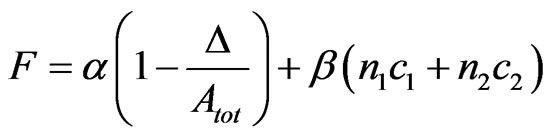 (4)
(4)
where:
• Atot = grid’s total area
• Δ is the covered area after the resources’ positioning
• n1 and n2 are respectively the number of the active resources with coverage ray R1 and the number of active resources with coverage ray R2.
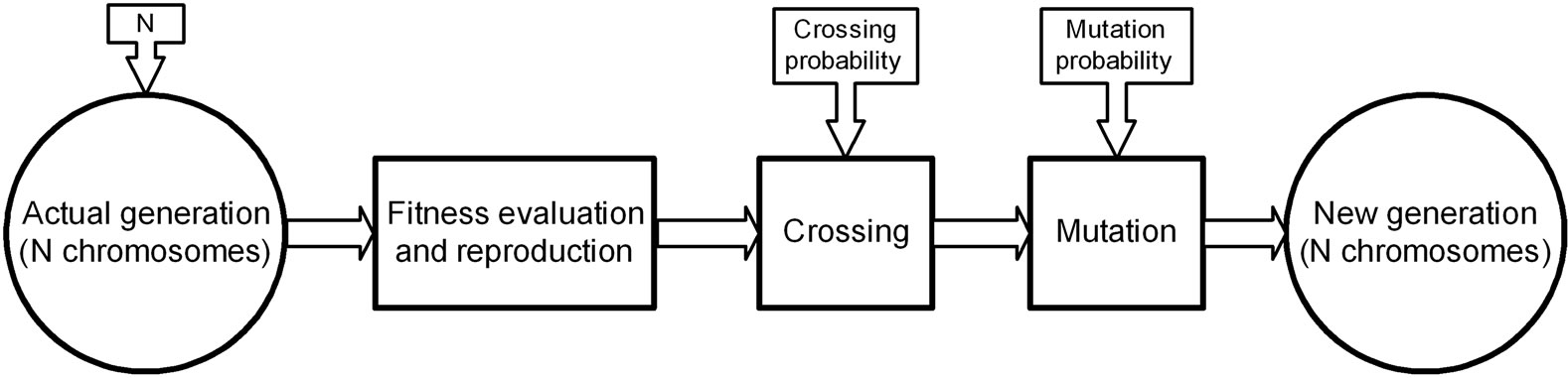
Figure 6. Operative scheme of a GA iteration.
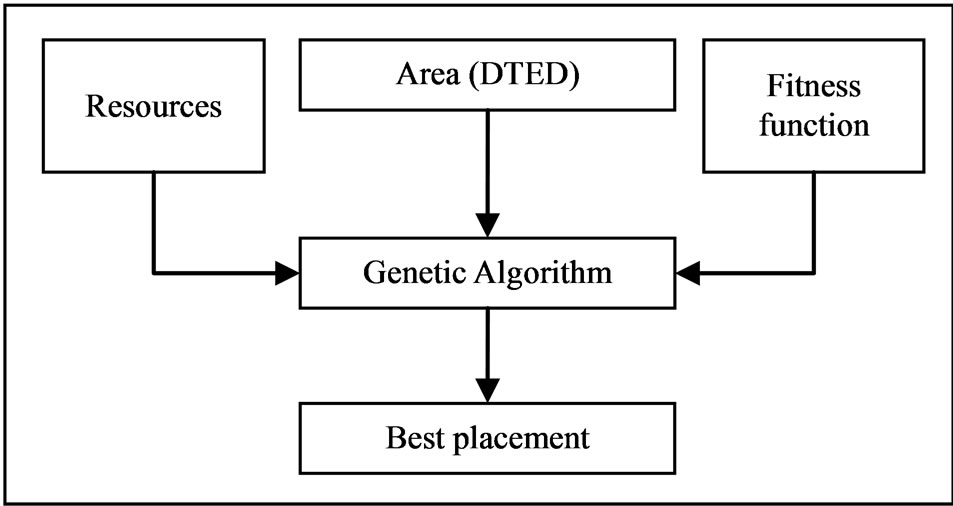
Figure 7. Solution’s scheme.
• c1 and c2 are factors associated to the resources that represent their cost.
• α and β are coefficients that allow to weigh properly the objective-function’s terms. Their evaluation is illustrated in the following.
In this case α and β are estimated by giving the condition that a resource should be added in the grid if it gives a contribution to the coverage at least equal to a percentage δ of its own coverage capability.
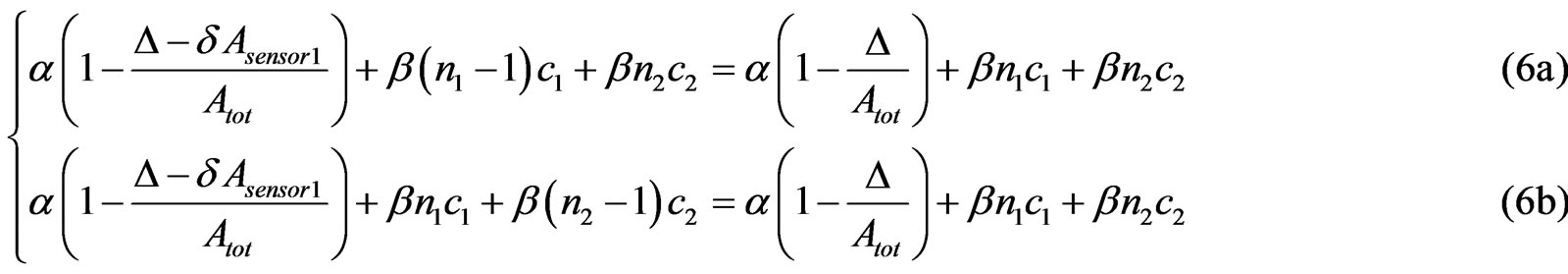
These coefficients can be estimated by solving the system below:
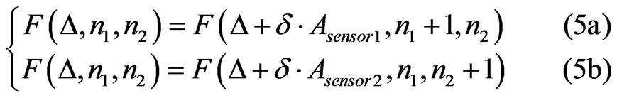
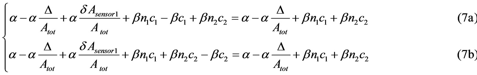
These equations give the equality between the objective-function’s value and the value of itself calculated by adding a new resource that gives a contribute to the total coverage percentage with a δ percentage of its own coverage capability. By this way it is possible to estimate the values of α and β that allow to eliminate resources which work under the minimum percentage. So it’s possible to reach the system below:
Solving this system it’s possible to obtain:
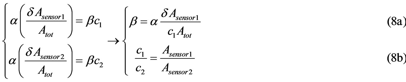
From these last equations it is possible to draw two important considerations. The first one is that the values of α and β aren’t bounded to a specific number so it’s possible to choose arbitrary values to be assigned to one of them and obtain the value of the other one by Equation (8a). The second consideration comes from the analysis of Equation (8b) where it’s possible to see how the resource’s cost is directly proportional to the coverage area of the resource itself. To calculate effective values of these parameters it’s necessary to express the objective-function with other parameters.
Dividing all the terms of Equation (8b) by the total area we obtain:
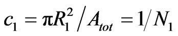 (9a)
(9a)
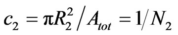 (9b)
(9b)
where N1 and N2 are respectively the maximum number of resources with ray R1 and the maximum number of resources with ray R2. Replacing these values in Equations (8a) and (8b) we obtain:
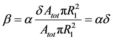 (10)
(10)
As it can be seen, the value of β depends on the minimum percentage δ that the resources must have to remain placed in the grid. Considering a real working percentage of the order of 40%, we obtain δ = 0.4. Replacing this value in the previous equation we have:
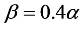 (11)
(11)
At this point it is necessary to calculate the value of α to find the final values of these parameters. The objective-function’s values must be included in a range [0, 1], where 1 represents the worst case and 0 the best case in which the 100% of coverage and the minimum use of resources is reached. Considering the condition for the worst case, it’s possible to estimate the value of α. In fact, in the worst case, no resource is placed on the grid so the coverage percentage is 0. Replacing these values in the objective-function we obtain:
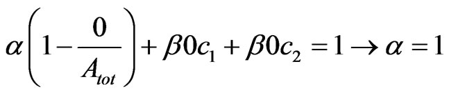 (12)
(12)
Finally the values of α and β are:
Replacing these values in Equation (4) we obtain:
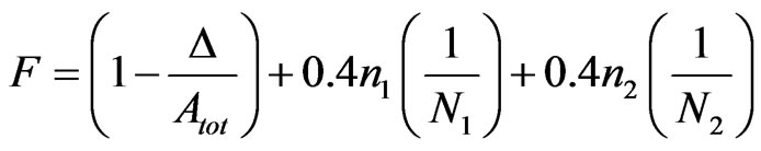 (14)
(14)
Analysing this function it’s possible to draw the considerations below:
• if no resources are placed on the grid (n1 = 0 and n2 = 0), the value of Equation (14) is equal to 1.
• if the coverage area is 100% it’s difficult to establish which is the fitness value. In this case the first term is equal to 0 while the sum of the other two has a value that is impossible to know a priori. If we consider that using all the resources the fitness value is equal to 0.8, it’s simple to understand that in the case of total coverage the fitness value is lesser than this number.
• how it can be seen, the resources used to cover the grid are weighed with the inverse of their maximum number so directly with the square of their own coverage ray: a resource with longer coverage ray weights in a more negative way on the fitness value with respect to a resource with shorter coverage ray.
This function allows the algorithm to eliminate resources which have been placed on the grid but that because of superimpositions or because of presence of obstacles can’t give a contribute to the coverage that is at least equal to the 40% of their own coverage capability and the single terms weight on the final fitness value is now calculated. Starting from the first element, it’s possible to estimate how much an increase of the coverage percentage of 1% weighs on the fitness value. To estimate it, it’s necessary to calculate the difference between the first term with no coverage and the first term with 1% of coverage:
 (15)
(15)
An increase of one point of percentage reflects on the fitness value with a decrease equal to 0.01.
To estimate the weight of the other two terms it’s sufficient consider only one kind of resource. One resource with coverage ray R1 weighs on the fitness value with a value W1 equal to:
 (16)
(16)
so its contribution, as just said, depends on its ray.
Similarly for a resource with coverage ray R2 is:
 (17)
(17)
Comparing Equation (16) and Equation (17) it is possible to see that adding one resource with coverage ray R1 weighs more than adding a resource with coverage ray R2.
4.2. Places Choice
To complete this work is possible to consider the sites that can be utilized to place the resources. By an a-priori analysis of the grid it is possible to find those sites that are non-reachable or that are occupied by other resources previously placed. After doing this analysis, a matrix is generated. The matrix is as big as the grid to cover. The sites that can’t be used are marked with a logical 0. If a resource is placed on a 0, the related solution is deleted by a penalization of its fitness value.
5. Performances and Results
5.1. Evaluation Time
In this section an approximation of the computation time is done, to estimate the time necessary to obtain a configuration closer to a real situation. The first consideration to do is that the most of the time is spent by the genetic algorithm to evaluate the objective-function and above all to evaluate the resource’s coverage; the classic genetic operations such as coding, selection, crossover and mutation can be considered instantaneous so they aren’t considered in this calculus. Therefore we consider only the function that evaluates the coverage and it’s possible to consider the calculus of a single cell as a unit-operation. The number of the cells that is evaluated depends on the resource’s ray and on the angular and radial steps that are chosen for the evaluation. It’s necessary to consider that this number could be smaller because of the obstacles on the grid. The number of unit-operation (Nop) for the evaluation of a single resource is:
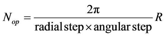 (18)
(18)
It is possible to see that the number of unit-operations depends directly on the ray and inversely on the radial step (the step on which we move along a radial direction) and on the angular step (angular distance between two subsequent radials). In this case we used a radial step equal to 1 for the coverage’s estimation.
Now it is necessary to insert this calculus in the context of the genetic algorithm in which every coverage’s calculus of a resource is applied to every active resource for every chromosome of every generation. Starting with considering active resources in a chromosome, we have the number of unit-operations for every chromosome (Nopch):
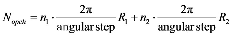 (19)
(19)
where n1 and n2 are respectively the number of active resources with coverage ray R1 and active resources with coverage ray R2 in a single chromosome. To obtain the number of unit-operation in a generation (Nopgen) it’s necessary to sum this quantity for every chromosome in a generation:
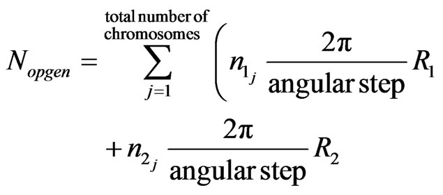 (20)
(20)
where and
and  are respectively the number of active resources with coverage ray R1 and the number of active resources with coverage ray R2 in the chromosome j.
Now, to obtain the total number of unit-operations in a cycle (Nopc), it’s necessary to execute the sum on every generation:
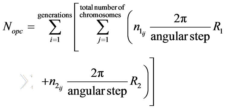 (21)
(21)
where  and
and  are respectively the number of active resources with coverage ray R1 and the number of active resources with coverage ray R2 in the j chromosome and in the i generation.
How we can see, the number of operations that it’s necessary to do is directly proportional to the ray of the resource and inversely proportional to the chosen angular step. Naturally this number depends on the number of chromosomes and generations. If we want to reduce the calculus time we have to reduce the generations’ number, the chromosomes’ number, the resource’s ray or we have to increase the radial or angular step. Each operation makes the algorithm faster but has a negative effect on the final solution so it’s necessary to find the right compromise between computation time and solution’s goodness.
Now we analyse the curve that represents the time trend as a function of the grid to explore.
We consider a starting grid of n*n in which are placed resources with area A1 and A2. The initial number of the resources is given by:
 (22a)
(22a)
 (22b)
(22b)
If we increase the grid side we can have two different cases: in the first case the ratio between total area and resource area remains equal while in the second one the resources area remain equal.
For the first case we want to double the side grid obtaining a 2n * 2n grid. The total area of the grid is 4n2.
If we increase not only the side grid but also the resources areas, keeping constant the number of initial resources, we obtain:
 (23)
(23)
where  is the number of resources with area
 .
.
This quantity must be equal to Equation (22a) and Equation (22b) because we supposed that the ratio between resource area and total area is equal, keeping unchanged the number of initial resources, so it must be . Similarly, for the other resource, it’s
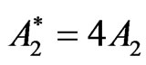 . With this argument it’s simple to understand that resources areas are multiplied by four as the number evaluated cells and the number of unit-operations. Analysing the second case, the resources areas are constant while the grid side is multiplied for a factor two. In this situation the number of initial resources increases according to the equations:
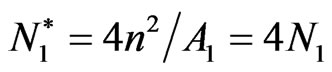 (24a)
(24a)
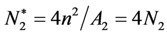 (24b)
(24b)
where  is the number of initial resources in the grid with side 2n. How we can see in this case, the number of initial resources is multiplied by four increasing in the same way the number of unit-operations.
Summarizing, in both of cases if the grid side is duplicated, the number of unit-operations is multiplied for four. The same is valid for every factor we multiplied the grid side: the number of unit-operations, and therefore the computational time, is multiplied by the square of that factor according to the equation below:
 (25)
(25)
where T1 is the time spent for evaluating the starting grid, L1 is the starting grid side, L2 is the new grid side and T2 is the time spent to evaluate the new grid.
Evaluation time increases in quadratic way with respect to the expansion grid side factor and is characterized by the trend shown in Figure 8.
In this graphic two points are signed: the first is the point that represents the grid configuration we used in the simulations and we use it as a point of reference. The second point is that one that represents a situation closer to reality in which the expansion grid side factor is 80. In this last case the computation time is equal about to 9 hours, as it is possible to see in the graphic.
5.2. Convergence of Solutions
Solution convergence is different depending on the parameters’ configuration that is used. In Figure 9 fitness graphics as a function of generation number for different cases we studied (Table 1) are shown.
It is possible to see that trends are very different from each other: some of them converge very early while other configurations don’t converge in the first 100 generations. It’s possible to affirm that every configuration reach the same final result but some of them reach it faster than others so these configurations are the best because they allow us to decrease evaluation time. For this study we considered 500 generations but for some configurations it is possible to decrease the number of generations up to 250 halving evaluation time, so this figure considers only the first 250 generations.
An example of solution is shown in Figure 10.
6. Numerical Results
In Table I the mean values of all the studied situations are reported so it is possible make a comparison between each other. The first 10 situations are evaluated without obstacles on the grid to test and verify the goodness of the genetic algorithm. The situations from 11 to 20 are evaluated considering the example DTED data shown in Figure 11. A 50 km * 50 km territory is considered; each cell is 1 km * 1 km and the angular step for coverage verification is 30˚.
In the first part of the table the values extracted at the generation number 250 are reported while in the second part the values extracted at the end of the genetic cycle are reported.
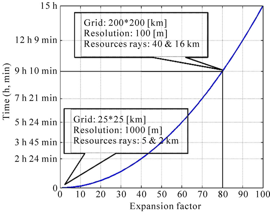
Figure 8. Trend of the evaluation time according to the grid’s expansion factor using a 2800 MHz PC, Intel CPU Pentium IV.
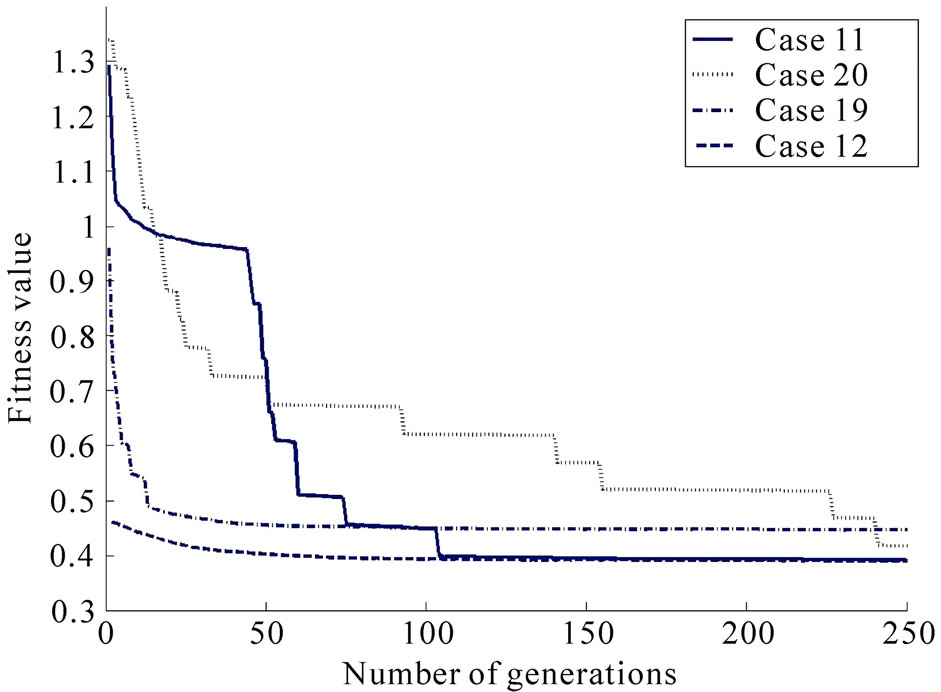
Figure 9. First 250 generations of the most interesting cases.
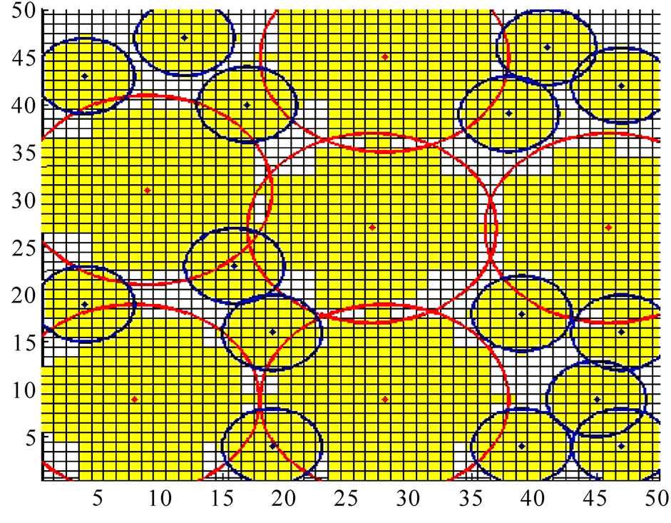
Figure 10. Example of solution: coverage of a [50 km * 50 km] grid with a 30˚ angular step using R1 = 10 km and R2 = 4 km, case 18 of table 1, grid step = 1 km.
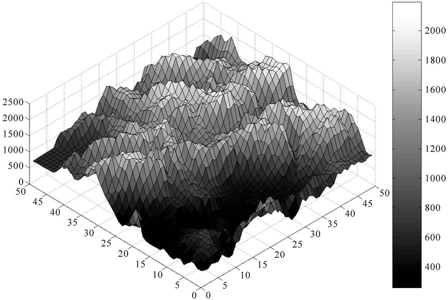
Figure 11. 3D-DTED level 0 used for simulations.
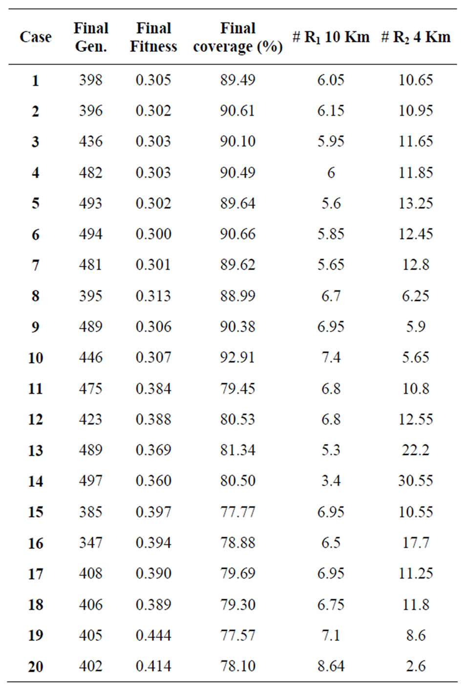
Table 1. Numerical results of different cases.
How we can see from this table, every configuration is characterized by similar performances about the final coverage percentage and the final fitness value in the two parts of the table. The difference between them is represented by the number of generations necessary to reach the final solution: in some cases the configurations use a low number of generations so they reach the final solution in a shorter time with respect to other configurations.
7. Conclusions
At the end of this work some considerations are possible. The first is that the genetic algorithm shown its strength of application in the resolution of complex problems such as the one we considered. It can solve real problems because it can consider all their practical characteristics (DTED, resources with different coverage ray R, etc.).
The algorithm has shown to be extremely flexible and it can be used to solve other complex problems.
This work shows that an efficient automation of the process of territorial resources placement is possible.
The resolution of the problem by the genetic algorithm gives good results: the genetic algorithm is very adaptable to this problem. The algorithm has demonstrated to be useful since it can find always good solutions. The important consideration to draw is that the goodness of the solutions depends on the variations of the configurations but it’s important to remember that best solutions require more time to be found so it’s necessary to find a compromise between solutions goodness and computation time.
In this work different implementations of the algorithm have been studied to try to improve its performances. The main implementations were directed to insert an a-priori knowledge: the reduction of the number of resources with coverage ray R2 and the insertion of a non-random initial population has shown a significant importance in the improvement of the results. Not all the simulations gave optimal solutions (such as the different kind of crossover and mutation that were implemented ad-hoc).
For future work and above all for future study of this problem, it’s possible to extend this work in a wider region using more efficient techniques to reduce the evaluation time such as the memorization of the visibility of the cells.
REFERENCES
- S. S. Dhillon, K. Chakrabarty and S. S. Iyengar, “Sensor Placement for Grid Coverage under Imprecise Detections,” Proceedings of the 5th International Conference on Information Fusion, Vol. 2, 8-11 July 2002, pp. 1581- 1587.
- K. Chakrabarty, S. S. Iyengar, H. Qi and E. Cho, “Grid Coverage for Surveillance and Target Location in Distribuited Sensor Networks,” IEEE Transactions on Computers, Vol. 51, No. 12, 2002, pp. 1448-1453. doi:10.1109/TC.2002.1146711
- S. Liu, Y. Tian and J. Liu, “Multi Mobile Robot Path Planning Based on Genetic Algorithm,” Proceedings of the 5th World Congress on Intelligent Control and Automation, Vol. 5, 15-19 June 2004, pp. 4706-4709.
- F. Garzia and R. Cusani, “Optimization of Cellular Base Stations Placement in Territory with Urban and Environmental Restrictions by Means of Genetic Algorithms,” Proceedings of Environment and Technological Innovation Energy, Rio de Janeiro, 2004.
- F. Garzia, C. Perna and R. Cusani, “UMTS Network Planning Using Genetic Algorithms,” International Journal of Communications and Network, Vol. 2, No. 3, 2010, pp. 193-199.
- H. Maini, K. Mehrotra, C. Mohan and S. Ranka, “Knowledge-Based Non-Uniform Crossover,” Proceedings of the First IEEE Conference on Evolutionary Computation, IEEE World Congress on Computational Intelligence, Orlando, 27-29 June 1994, pp. 22-27. doi:10.1109/ICEC.1994.350048
- E. Falkenauer, “The Worth of the Uniform,” Proceedings of Congress on Evolutionary Computation, Vol. 1, 6-9 July 1999, pp. 138-146.
- L. J. Zhang, Z. H. Mao and Y. D. Li, “Mathematical Analysis of Crossover Operator in Genetic Algorithms and Its Improved Strategy,” Proceedings of IEEE International Conference on Evolutionary Computation, Perth, Vol. 1, 29 November-1 December, 1995, pp. 412-222. doi:10.1109/ICEC.1995.489183
- Y. Shang and G. J. Li, “New Crossover Operators in Genetic,” Proceedings of the Third International Conference on Tools for Artificial Intelligence, 10-13 November 1991, pp. 150-153. doi:10.1109/ICEC.1995.489183
- J. Lu, B. Feng and B. Li, “Finding the Optimal Gene Order for Genetic Algorithm,” Proceedings of the 5th World Congress on Intelligent Control and Automation, Vol. 3, 15-19 June 2004, pp. 2073-2076. doi:10.1109/WCICA.2004.1341949
- G. Bilchev, H. S. Olafsson and L. Comparino, “Genetic Algorithms and Greedy Heuristics for Adaptation Problems,” Proceedings of IEEE International Conference on Evolutionary Computation, IEEE World Congress on Computational Intelligence, 4-9 May 1998, pp. 458-463.
- J. A. Vasconcelos, J. A. Ramirez, R. H. C. Takahashi and R. R. Saldanha, “Improvements in Genetic Algorithms,” IEEE Transactions on Magnetics, Vol. 37, No. 5, 2001, pp. 3414-3417. doi:10.1109/20.952626
- K. Y. Chan, M. E. Aydin and T. C. Fogarty, “An Epistasis Measure Based on the Variance for the Real-Coded Representation in Genetic Algorithms,” Proceedings of Congress on Evolutionary Computation, Vol. 1, 8-12 December 2003, pp. 297-304.
- M. O. Odetayo, “Empirical Study of the Interdependencies of Genetic Algorithms Parameters,” Proceedings of the 23rd EUROMICRO Conference, New Frontiers of Information Technology, Budapest, 1-4 September 1997, pp. 639-643.
- J. Cheng, W. Chen, L. Chen and Y. Ma, “The Improvement of Genetic Algorithm Searching Performance,” Proceedings of International Conference on Machine Learning and Cybernetics, Vol. 2, 4-5 November 2002, pp. 947-951.
- Z. Wang, D. Cui, D. Huang and H. Zhou, “A Self-Adaptation Genetic Algorithm Based on Knowledge and Its Application,” Proceedings of 5th World Congress on Intelligent Control and Automation, Vol. 3, 15-19 June 2004, pp. 2082-2085. doi:10.1109/WCICA.2004.1341951
- H. Shimodaira, “A New Genetic Algorithm Using Large Mutation Rates and Population-Elitist Selection (GAL ME),” Proceedings of the 8th IEEE International Conference on Tools with Artificial Intelligence, 16-19 November 1996, pp. 25-32.
- S. Ghoshray and K. K. Yen, “More Efficient Genetic Algorithm for Solving Optimization Problems,” Proceedings of IEEE Interantional Conference on Systems, Man and Cybernetics, Intelligent System for the 21st Century, Vol. 5, 22-25 October 1995, pp. 4515-4520.
- M. R. Akbarzadeh and T. M. Jamshidi, “Incorporating A-Priori Expert Knowledge in Genetic Algorithms,” Proceedings of IEEE International Symposium on Computational Intelligence in Robotics and Automation, 10-11 July1997, pp. 300-305.
- N. Chaiyaratana and A. M. S. Zalzala, “Recent Developments in Evolutionary and Genetic Algorithms: Theory and Applications,” Proceedings of the 2nd International Conference on Genetic Algorithms in Engineering Systems: Innovations and Applications, 2-4 September 1997, pp. 270-277.
- D. E. Goldberg, “Genetic Algorithms in Search, Optimization and Machine Learning,” Addison-Wesley, Boston, 1989.
- L. Nagi and L. Farkas, “Indoor Base Station Location Optimization Using Genetic Algorithms,” Proceedings of IEEE International Symposium on Personal, Indoor and Mobile Communications, London, Vol. 2, 2000, pp. 843- 846.
- B. Di Chiara, R. Sorrentino, M. Strappini and L. Tarricone, “Genetic Optimization of Radio Base-Station Size and Location Using a GIS-Based Frame Work: Experimental Validation,” Proceedings of IEEE International Symposium of Antennas and Propagation Society, Vol. 2, 2003, pp. 863-866.
- J. K. Han, B. S. Park, Y. S. Choi and H. K. Park, “Genetic Approach with New Representation for Base Station Placement in Mobile Communications,” Proceedings of IEEE Vehicular Technology Conference, Atlantic City, Vol. 4, 2001, pp. 2703-2707.
- R. Danesfahani, F. Razzazi and M. R. Shahbazi, “An Active Contour Based Algorithm for Cell Planning,” Proceedings of IEEE International Conference on Communications Technology and Applications, 2009, pp. 122-126. doi:10.1109/ICCOMTA.2009.5349224
- R. S. Rambally and A. Maharajh, “Cell Planning Using Genetic Algorithm and Tabu Search,” Proceedings of International Conference on the Application of Digital Information and Web Technologies, Beijing, 16-18 October 2009, pp. 640-645.
- K. Lieska, E. Laitinen and J. Lahteenmaki, “Radio Coverage Optimization with Genetic Algorithms,” Proceedings of IEEE International Symposium on Personal, Indoor and Mobile Radio Communications, Boston, Vol. 1, 8-11 September 1998, pp. 318-322.
- A. Esposito, L. Tarricone and M. Zappatore, “Software Agents: Introduction and Application to Optimum 3G Network Planning,” IEEE Antennas and Propagation Magazine, Vol. 51, No. 4, 2009, pp. 147-155. doi:10.1109/ICCOMTA.2009.5349224
- L. Shaobo, P. Weijie, Y. Guanci and C. Linna, “Optimization of 3G Wireless Network Using Genetic Programming,” Proceedings of International Symposium on Computational Intelligence and Design, Changsha, Vol. 2, 12-14 December 2009, pp. 131-134.
- C. Maple, G. Liang and J. Zhang, “Parallel Genetic Algorithms for Third Generation Mobile Network Planning,” Proceedings of International Conference on Parallel Computing in Electrical Engineering, 7-10 September 2004, pp. 229-236. doi:10.1109/ICCOMTA.2009.5349224
- I. Laki, L. Farkas and L. Nagy, “Cell Planning in Mobile Communication Systems Using SGA Optimization,” Proceedings of International Conference on Trends in Communications, Bratislava, Vol. 1, 4-7 July 2001, pp. 124- 127.
- D. B. Webb, “Base Station Design for Sector Coverage Using a Genetic Algorithm with Method of Moments,” Proceedings of IEEE International Symposium of Antennas and Propagation Society, Vol. 4, 20-25 July 2004, pp. 4396-4399.
- A. Molina, A. R. Nix and G. E. Athanasiadou, “Optimised Base-Station Location Algorithm for Next Generation Microcellular Networks,” Electronics Letters, Vol. 36, No. 7, 2000, pp. 668-669. doi:10.1049/el:20000515
- G. Cerri, R. De Leo, D. Micheli and P. Russo, “BaseStation Network Planning Including Environmental Impact Control,” IEEE Proceedings on Communications, Vol. 151, No. 3, 2004, pp. 197-203. doi:10.1049/ip-com:20040146
- A. Molina, G. E. Athanasiadou and A. R. Nix, “The Automatic Location of Base-Stations for Optimized Cellular Coverage: A New Combinatorial Approach,” IEEE International Conference on Vehicular Technology, Houston, Vol. 1, July 1999, pp. 606-610.
- N. Weaicker, G. Szabo, K. Weicker and P. Widmayer, “Evolutionary Multi-Objective Optimization for Base Station Transmitter Placement with Frequency Assignment,” IEEE Transactions on Evolutionary Computations, Vol. 7, No. 2, 2003, pp. 189-203. doi:10.1109/TEVC.2003.810760
- G. Fangqing, L. Hailin and L. Ming, “Evolutionary Algorithm for the Radio Planning and Coverage Optimization of 3G Cellular Networks,” International Conference on Computational Intelligence and Security, Beijing, Vol. 2, 11-14 December 2009, pp. 109-113.
- J. Munyaneza, A. Kurine and B. Van Wyk, “Optimization of Antenna Placement in 3G Networks Using Genetic Algorithms,” International Conference on Broadband Communications, Information Technology & Biomedical Applications, Gauteng, 23-26 November 2008, pp. 30-37.