Open Journal of Fluid Dynamics
Vol.3 No.2(2013), Article ID:33648,14 pages DOI:10.4236/ojfd.2013.32013
An Adaptive Response Compensation Technique for the Constant-Current Hot-Wire Anemometer
Department of Mechanical Engineering, Nagoya Institute of Technology, Nagoya, Japan
Email: *m.tagawa@nitech.ac.jp
Copyright © 2013 Soe Minn Khine et al. This is an open access article distributed under the Creative Commons Attribution License, which permits unrestricted use, distribution, and reproduction in any medium, provided the original work is properly cited.
Received February 9, 2013; revised March 10, 2013; accepted March 18, 2013
Keywords: Flow Measurement; Hot-Wire Anemometer; Turbulent Flow; Constant-Current Hot-Wire Anemometer; Response Compensation; Frequency Response; Time-Constant; Multipoint Measurement; Digital Signal Processing
ABSTRACT
An adaptive response compensation technique has been proposed to compensate for the response lag of the constant-current hot-wire anemometer (CCA) by taking advantage of digital signal processing technology. First, we have developed a simple response compensation scheme based on a precise theoretical expression for the frequency response of the CCA (Kaifuku et al. 2010, 2011), and verified its effectiveness experimentally for hot-wires of 5 μm, 10 μm and 20 μm in diameter. Then, another novel technique based on a two-sensor probe technique—originally developed for the response compensation of fine-wire thermocouples (Tagawa and Ohta 1997; Tagawa et al. 1998)—has been proposed for estimating thermal time-constants of hot-wires to realize the in-situ response compensation of the CCA. To demonstrate the usefulness of the CCA, we have applied the response compensation schemes to multipoint velocity measurement of a turbulent wake flow formed behind a circular cylinder by using a CCA probe consisting of 16 hot-wires, which were driven simultaneously by a very simple constant-current circuit. As a result, the proposed response compensation techniques for the CCA work quite successfully and are capable of improving the response speed of the CCA to obtain reliable measurements comparable to those by the commercially-available constant-temperature hot-wire anemometer (CTA).
1. Introduction
In recent years, particle image velocimetry (PIV) has become one of the most popular techniques for measuring velocity fields. The hot-wire anemometry [1-5], on the other hand, has long been used mainly for measuring turbulent gaseous flows because of its simple and highlyreliable measurement systems and wide range of applicability. Thus, the hot-wire anemometry is still frequently utilized as a reliable research tool for statistical and frequency analyses of turbulent flows.
The hot-wire anemometry is generally driven at three operation modes, i.e., the constant temperature, constantcurrent and constant voltage modes. For the application of the hot-wire anemometry, the constant-temperature anemometer (CTA) is commercially available and almost always used as a standard system for driving the hot-wire, while the other two modes are rarely used, primarily due to their response lag during velocity fluctuation measurement. However, the electric circuit of the CTA is not simple, and the measurement system is fairly expensive. On the other hand, the constant-current hot-wire anemometer (CCA) can be set up with a very simple and low-cost electric circuit for heating the hot-wire. Thus, if we improve the response characteristics of the CCA with the aid of digital signal processing, the CCA will have a great advantage over the CTA and will be a promising tool for multipoint turbulence measurement.
When a hot-wire is driven at a constant electric current, the wire temperature, which corresponds to the hot-wire output, does not respond correctly to high-frequency velocity fluctuations because of the thermal inertia of the wire. Thus, the CCA output needs to be compensated adequately for the response lag to reproduce high frequency components of the measurement data. In order to investigate the response characteristics of the hot-wire, Hinze [1] analyzed the dynamic behavior of the hot-wire with heat loss to the wire supports. As a result, it was shown that the aspect ratio of the hot-wire (the lengthto-diameter ratio) is an important parameter characterizing the response of the hot-wire. In our previous studies [6,7], we have successfully derived a precise theoretical solution for the frequency response of an actually-used hot-wire probe which consisted of a fine metal wire, stub parts (copper-plated ends/silver cladding of a Wollaston wire) and prongs (wire supports). As a result, we were able to find the geometrical conditions for the frequency response of the CCA to be approximated by the firstorder lag system, which can be characterized by a single system parameter called the thermal time-constant [5].
If the time-constant value is known in advance, we may apply the existing response compensation techniques for the first-order system [4,5] to recover the response delay in the CCA measurement. In reality, however, since the time-constant value of the CCA changes largely depending on flow velocity [8] and physical properties of the working fluid, it is very difficult to estimate the time-constant value of the hot-wire accurately. In our previous papers [6,7], we proposed a digital response compensation scheme based on the precise theoretical expression for the frequency response of the CCA. The results showed that the scheme worked successfully, reproducing high-frequency velocity fluctuations of a turbulent flow. However, this compensation scheme needs more information regarding the geometrical parameters of the hot-wire probe, i.e., the diameters and lengths of the wire and stub together with their physical properties.
In the present study, first, we thoroughly tested the theoretical expression for the frequency response of the CCA by applying it extensively to the digital response compensation of three different hot-wire probes consisting of tungsten wires 5 μm, 10 μm and 20 μm in diameter. Secondly, we have proposed a novel approach to the response compensation of the CCA output that will work without our knowing in advance the geometrical parameters of the hot-wire probe. This approach is based on a two-sensor probe technique for compensating the response delay of fine-wire thermocouples [9,10], and enables in-situ estimation of the time-constant values of the hot-wire probe, and will realize adaptive response compensation of the CCA outputs. Specifically, in the twosensor probe technique, two hot-wires of unequal diameters—having different response speeds—are used simultaneously, and the time-constant values of the two hotwires can be obtained from the measurement data itself without carrying out any dynamic calibration of the hotwire probe.
Finally, in order to demonstrate the usefulness of the CCA, we have applied the above response compensation schemes to multipoint velocity measurement of turbulent flows e.g., [11-13]. In the present multipoint measurement, we have simultaneously used 16 hot-wires driven by the CCA to measure a turbulent wake flow formed behind a cylinder. In these verification experiments, we have measured turbulence intensities (r.m.s. values), power spectra and instantaneous signal traces of the velocity fluctuations, and have compared them with those obtained by a hot-wire probe driven by a commercially available constant-temperature hot-wire anemometer.
2. Time Constant of Hot-Wire for CCA Mode
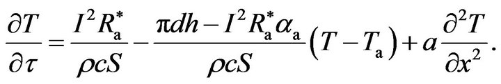
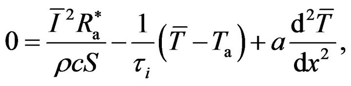
Figure 1 shows the geometrical features and coordinate system of the CCA probe used in the theoretical analysis (see Appendix A). As shown in Figure 1, the hot-wire is a fine tungsten wire (sensing part) with copper-plated ends (stubs) which are soldered to the prongs (wire supports). By applying electric current I to the fine-wire element (length: dx, diameter d1), the generated Joule heat should balance with the sum of the following heat losses: heat convection, heat conduction, heat accumulation and thermal radiation. Since the heated wire is very fine, we can assume that the amount of heat radiation is negligible and the cross-sectional temperature distribution is uniform [14]. Therefore, the energy balance equation for the hot-wire can be written as (in this section, the subscript 1 for wire or 2 for stub is omitted for simplicity):
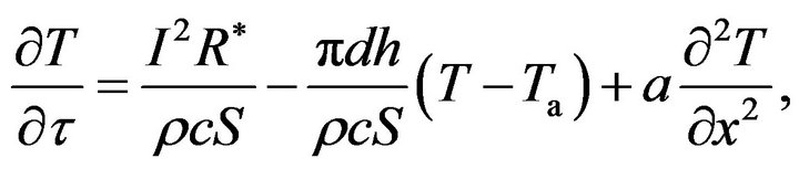 (1)
(1)
where t is time,  denotes the wire resistance per unit length and given by
 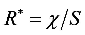 [c: electric resistivity,
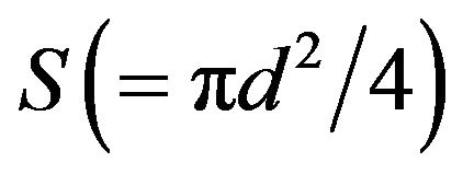 : cross-sectional area of the wire], and I: electric current, h: heat transfer coefficient, T: wire temperature, Ta: ambient fluid temperature,
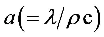 : thermal diffusivity of wire material, l: thermal conductivity, r: density, c: specific heat. In Equation (1),
  can be expressed as a linear function of the temperature difference between the wire and reference temperatures as:
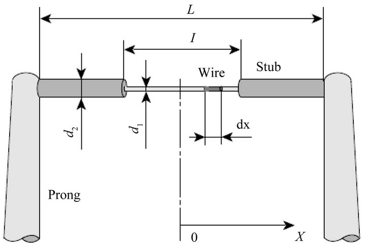
Figure 1. Geometrical features of hot-wire probe.
 (2)
(2)
where  is electric resistance per unit wire length at the reference temperature and aa denotes a temperature coefficient of wire material. Then, Equation (1) can be rewritten as:
 (3)
(3)
In hot-wire measurement, the effective cooling rate of the heated wire must principally be a function of flow velocity and can be obtained from the heat transfer coefficient of the fine wire, h, while the heat generation term is a nonlinear function of the electric current I and the wire resistance is determined by wire temperature as shown in Equation (2). To make Equation (3) theoretically treatable, it needs to be linearized by decomposing the relevant physical quantities into a time-averaged component and a fluctuation one as: 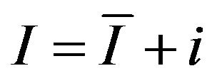
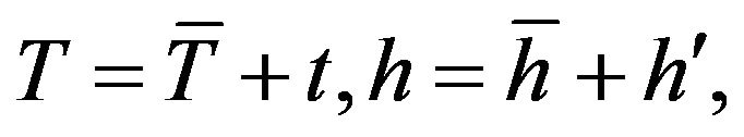 [1,15,16]. Then, we can obtain a governing equation of the constant-current hot-wire anemometer by formulating the energy balance equation with the following procedures: 1) ignore the contribution of the secondand higher-order fluctuation components; 2) derive a governing equation for the first-order fluctuation components by time-averaging the equation obtained in 1); 3) introduce a well-accepted correlation of
 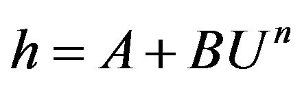 to relate the heat transfer coefficient to the flow velocity; and 4) assume the electric current I to be constant. From the above procedures, the static and dynamic characteristics of the CCA are expressed as:
 (4)
(4)
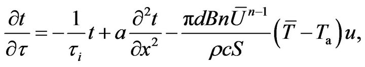 (5)
(5)
where  is the thermal time-constant (
 or 2), and is primarily related to the time-averaged heat transfer coefficient around the fine wire
  and electric current
  as follows:
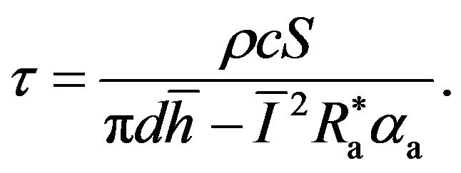 (6)
(6)
In Equation (6), the heat transfer coefficient  can be expressed as a function of flow velocity
  and is written as:
 (7)
(7)
where the constants A, B and n can be obtained from the Collis-Williams correlation equation [17]; see Equation (A13). As seen from Equation (6), the time constant ti should be a complex function of flow velocity , driving current
 , wire diameter d, etc. Thus, in general, we need to either obtain the time-constant value experimentally or estimate it empirically.
3. Response Compensation Techniques for the CCA
3.1. Response Compensation Based on Precise Frequency Response Function
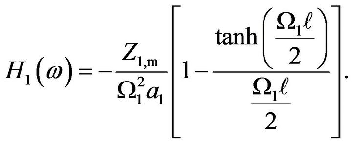
The frequency response of the hot-wire driven by the CCA,  , has been derived theoretically by the authors [6,7], and is expressed by the following equation
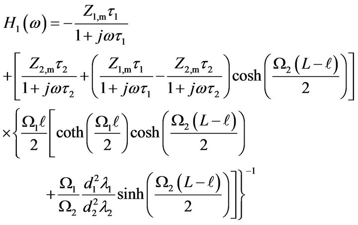
(8)
To estimate theoretically the frequency response of hot-wires, we have applied Equation (8) to the three different tungsten hot-wires (5 μm, 10 μm and 20 μm in diameter) with copper-plated ends (stubs). The geometrical parameters of the hot-wires are given in Table 1, in which ℓ/d1 and L denote the aspect ratio of the fine-wire and the distance between the prongs, respectively. All the hot wires have copper-plated ends 35 μm in diameter and are supported by the prongs (see Figure 1). In the present analysis, electric currents for the hot-wires driven at the CCA mode were set respectively at 40 mA, 100 mA and 260 mA for the 5 μm, 10 μm and 20 μm hot-wires, so as to provide adequate sensitivity to flow velocity. The airflow velocity and fluid temperature were 7 m/s and 25˚C, respectively. Figure 2 shows the Bode diagram (gain) calculated from Equation (8). As shown in Figure 2, the frequency response of the hot-wire driven at the CCA mode can be naturally improved by decreasing the wire diameter. In the present calculation conditions, the 5 μm tungsten wire responded adequately to velocity fluctuations up to about 100 Hz without response compensation, while the response speed of the 20 μm wire decreased by an order of magnitude compared with the 5 μm one.
The length-to-diameter ratio (aspect ratio) of the tungsten wires shown in Figure 2 ranges from 200 to 300. In this regard, Hinze [1] showed that, for platinum-iridium wires, the aspect ratio should be greater than 200, and be still higher for tungsten wires to make the wire resistance (temperature) almost uniform along the central 60 per-
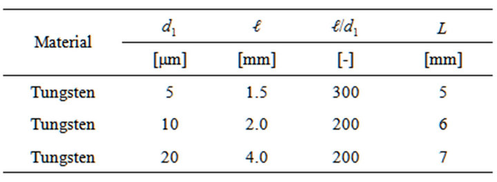
Table 1. Detailed features of three different hot-wires used. Definitions of the geometrical parameters d1, ℓ and L are given in Figure 1.
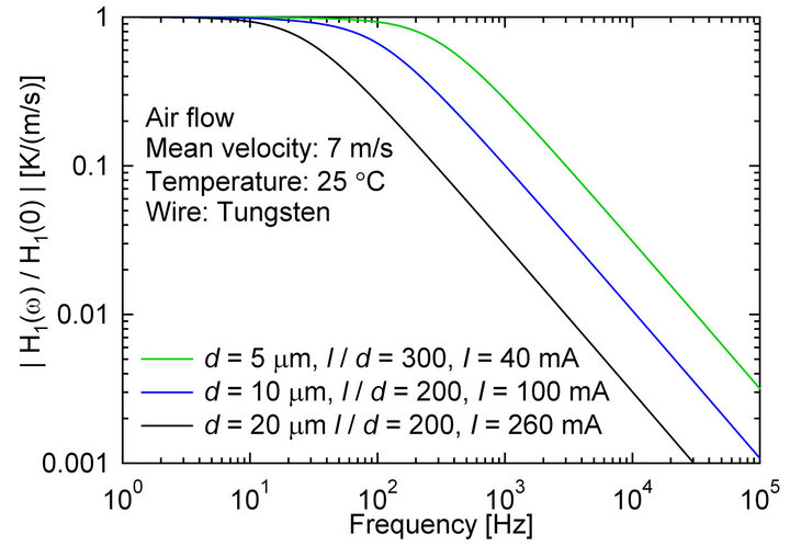
Figure 2. Frequency response of CCA obtained from Equation (8) as a function of length-to-diameter ratio (tungsten wires 5 μm, 10 μm and 20 μm in diameter). (see Appendix A).
cent of its length. In such a case, as seen from Figure 2, the frequency response of the hot-wire driven by the CCA can be approximated by the first-order lag system, whose response can be expressed as a function of only the time constant. If the aspect ratio becomes smaller than about 200, the cooling effects of the wire supports such as the stub and prong will emerge, and can deteriorate the frequency response of the hot-wire. As a result, the Bode diagram for shorter wires behaves in a more complex manner (see Figure A1 in Appendix A).
The digital signal processing of the response compensation based on a known frequency-response function was described in detail in a previous paper [10]. The procedure is applicable to the hot-wire measurement and can be summarized as follows: First, the hot-wire output (time-series data) is transformed into frequency-domain components using the fast Fourier transform (FFT). Next, each frequency component is multiplied by 1/H1 (w)— the reciprocal of Equation (8)—to compensate for the output in the frequency domain. Finally, the inverse FFT is applied to the frequency-domain components thus calculated to obtain the compensated time-series data of the hot-wire output.
3.2. Response Compensation of CCA by Two-Sensor Technique
To use the above response compensation scheme based on Equation (8), we need to know the geometrical parameters of the hot-wire probe. On the other hand, if the frequency response of the hot-wire can be represented by the first-order lag system, we can apply the two-sensor technique, which does not need the geometrical parameters of the probe [9,10], to the response compensation of the CCA. In the present study, we used two methods called  and
and . Their methods are given below.
3.2.1. emin Method
The first-order lag systems of the two hot-wires driven by the CCA can be expressed as follows:
 (9)
(9)
where Ui and Ug denote respectively raw output of the CCA (uncompensated velocity) and fluid velocity around the hot-wire, and t and ti are the time and time-constant defined by Equation (6), respectively. The subscripts  and 2 denote two unequal hot-wires different in diameter. Ideally, the fluid velocities surrounding the two hot-wires, Ug1 and Ug2, must be expressed as
  . In reality, however, the finite spatial resolution between the two hot-wires and the instrumentation noise may change the relation between Ug1 and Ug2 as
 . Thus, the time constants t1 and t2 can be determined so as to minimize the mean square value of the difference between Ug1 and Ug2, which is given by
 (10)
(10)
The time-constant estimation method thus obtained was originally proposed by Tagawa and Ohta [9]. In what follows, we call this estimation scheme the “emin method”. Then, the time constants t1 and t2 can be obtained from the simultaneous equation derived from Equation (10) by minimizing the value of e. The result is given by the following equations:
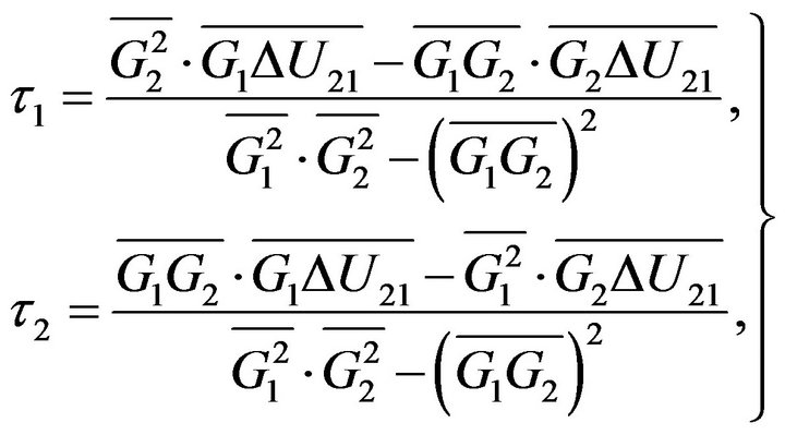 (11)
(11)
where G is the time derivative of  and
and .
.
3.2.2. Rmax Method
In a case where there is a low spatial resolution of the two-sensor probe and/or a low signal-to-noise ratio of the measurement system, we can take another approach to estimate the time-constant values by maximizing the correlation coefficient R between Ug1 and Ug2:
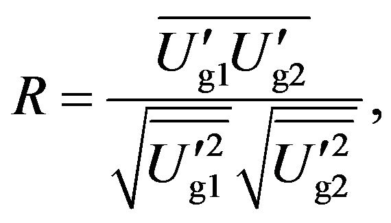 (12)
(12)
where the prime denotes a fluctuating component. By solving a simultaneous equation thus derived, we obtain the time constants t1 and t2 as a solution of quadratic equations:
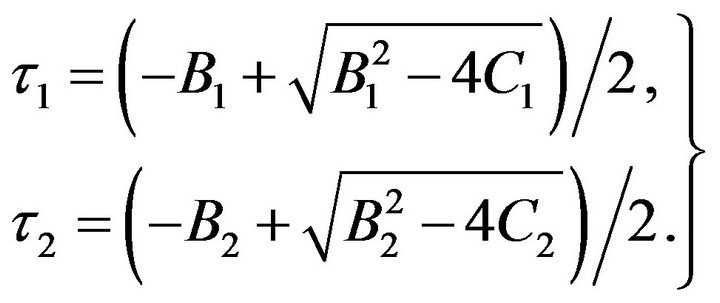 (13)
(13)
The quantities  and C2 in Equation (13) are given by
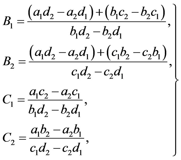 (14)
(14)
and all the elements in Equation (14) are given by
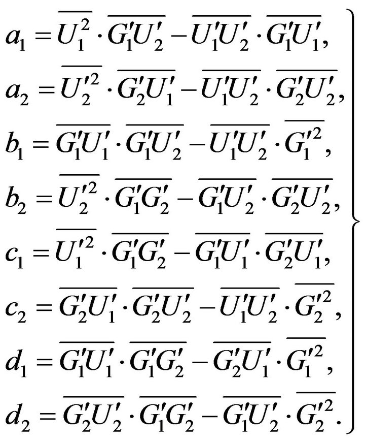 (15)
(15)
In the present study, we have mainly used this approach called the “Rmax method” [10]. It is noted that the time derivatives in Equations (11) and (15) can be obtained from the coefficients of a polynomial curve-fitting [18] for the digitized outputs of the two unequal hotwires driven at the CCA mode.
4. Experimental Apparatus and Measurement System
4.1. Single-Sensor and Two-Sensor Probes
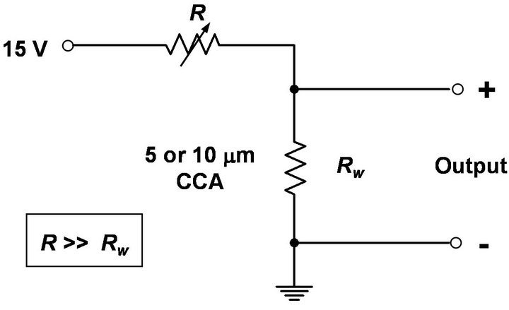
In this experiment, we used three fine tungsten wires 5 μm, 10 μm and 20 μm in diameter for the CCA, and a 5 μm tungsten wire for the CTA, which was used as a reference sensor. The detailed features of the fine-wires are given in Table 1. For the two-sensor technique, we have constructed two types of the CCA probes—one is the combination of 5 and 10 μm hot-wires, and the other is that of 10 and 20 μm ones. The schematic diagram of the constant-current circuit for driving a 5 μm or 10 μm wire is shown in Figure 3(a), and that for a 20 μm wire in Figure 3(b). The driving circuit for 5 μm and 10 μm wires is very simple and can be composed at quite a low cost. On the other hand, a different circuit (shown in Figure 3(b)) should be used for a 20 μm wire, since the current needs to be kept accurately constant even in case of a higher electric current. The later circuit, of course, can be used for driving a thinner wire, and is still much simpler to operate than the constant-temperature anemometer. The configuration and arrangement of the hotwires consisting of single-sensor and two-sensor probes are shown (circled) in Figure 4. We have determined a proper wire separation so as to minimize thermal and
 (a)
(a)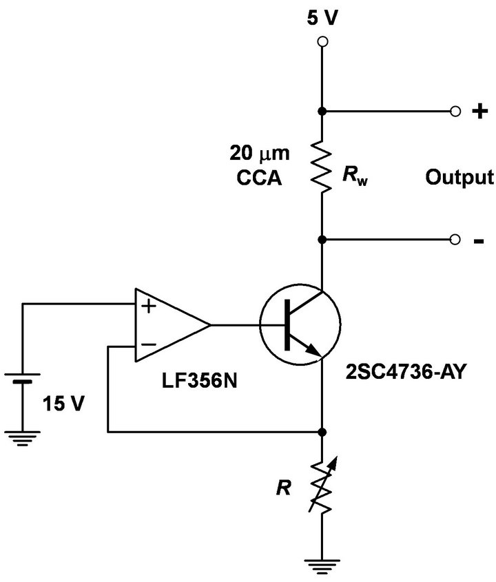 (b)
(b)
Figure 3. Schematic diagrams of constant-current circuits for driving three different tungsten hot-wires 5, 10 and 20 μm in diameter: (a) Driving circuit for 5 and 10 μm wires. Resistance values Rw of 5 μm wire (length: 1.5 mm) and 10 μm one (length: 2 mm) are 5.5 - 6.5 Ω and 2 - 3 Ω, respectively, at room temperature. Driving currents for 5 μm and 10 μm wires were 40 mA and 100 mA, respectively; (b) Driving circuit for 20 μm wire. The resistance value Rw of 20 μm wire (length: 4 mm) is 1 - 2 Ω at room temperature. The driving current was 260 mA.
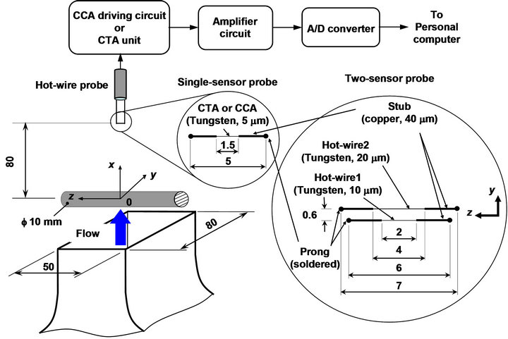
Figure 4. Experimental apparatus and details of hot-wire probes (single-sensor and two-sensor probes). The 10 μm and 20 μm hot-wire sensors shown in the two-sensor probe can be used for the single-sensor probe. For the two-sensor probe, we employed two combinations: Probe 1 is the combination of 5 μm and 10 μm hot-wires; Probe 2 (circled) is that of 10 μm and 20 μm ones. (All dimensions in millimeters.)
fluid-dynamical interferences between the two hot-wires.
4.2. Experimental Apparatus and Measurement System
As shown in Figure 4, the flow field to be measured is a turbulent far wake of a circular cylinder, and the test section is the  mm region in the central plane
  at
at . A uniform airflow up to 12 m/s can be produced using an upright wind tunnel with a two-dimensional contraction (contraction ratio, 5:1), and approaches to the cylinder set at the wind tunnel exit. It is noted that 5% - 10% free stream turbulence is generated by a perforated plate (hole size:
  5 mm; staggered arrangement with 7 mm pitch). In the present experiment, the uniform airflow velocity was set to 7 m/s.
All the outputs of the hot-wires driven by the constantcurrent circuits shown in Figure 3 are amplified by 100 - 500 times and digitized by a 14-bit A/D converter (Microscience ADM-670 and/or 681PCI). The sampling frequency is set at 10 kHz and the number of samples is 132,000 for each measurement. A personal computer (EPSON Endeavor Pro3100) is used to store the hot-wire outputs of the A/D converter and perform all the data processing. The hot-wire outputs are calibrated with the aid of a pitot tube in the range of 1 to 10 m/s.
5. Results and Discussion
5.1. Theoretical Response Compensation for Single-Sensor Measurement
First, we estimated the frequency response of the hotwires 5 μm, 10 μm and 20 μm in diameter to apply the theoretical response compensation scheme mentioned in section 3.1 to the CCA outputs.
Naturally, the mean velocity profiles obtained by these three hot-wires show little difference (a sample velocity profile is seen in Figure 5). Then, we appraised experimentally the effectiveness of the theoretical response compensation of the CCA on the basis of the turbulence intensities (root-mean-square values) and power spectra of the velocity fluctuations of the turbulent wake flow. The results are shown in Figures 6 and 7. Figure 6 shows the root-mean-square (r.m.s.) velocities of the uncompensated (raw) and compensated CCA outputs in comparison to the CTA results used as reference data. As seen from Figure 6, all the three compensated r.m.s. profiles are generally in good agreement with the CTA data. On the other hand, Figure 7" target="_self"> Figure 7 shows the uncompensated and compensated power spectra of the CCA data measured at y = 16 mm, where the r.m.s. profiles indicate the peak values. As seen from the comparison between the uncompensated and compensated power spectra, the CCA outputs start to attenuate at about 200 Hz, 70 Hz and 20 Hz for the 5 μm, 10 μm and 20 μm hot-wire data, respectively. These behaviors of the uncompensated power spectra can be well explained by the Bode (gain) diagrams shown in Figure 2, and the compensated power spectra agree well with the CTA result up to sufficiently high-frequencies. It is noted that, in the present study, we have applied a finite-impulse-response (FIR) digital filter to the compensated CCA outputs in order to cut off the frequency components higher than 4.5 kHz, 3 kHz and 2 kHz for the 5 μm, 10 μm and 20
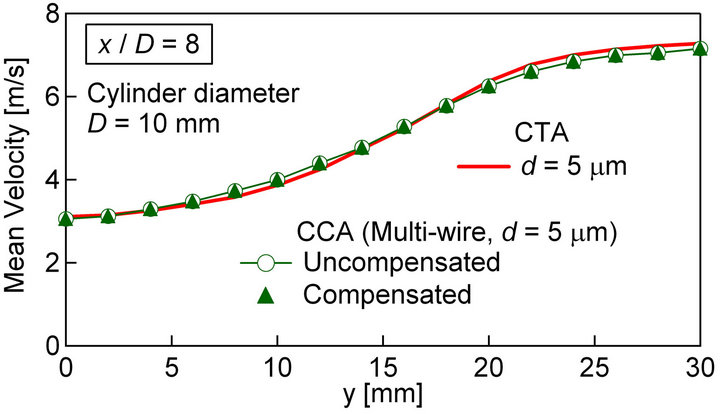
Figure 5. Mean velocity profiles of single-sensor measurement by CTA and multipoint measurement by CCA (see Section 6.2). Cylinder is positioned at y = 0 mm.
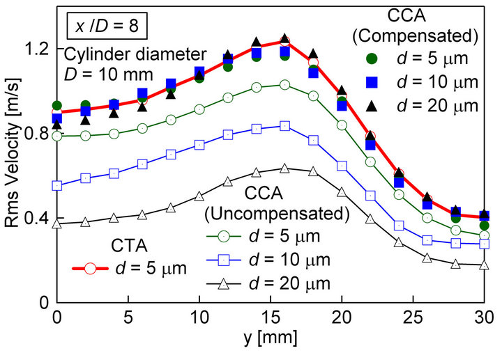
Figure 6. Comparison of rms velocity profile between single-wire CCA measurements by 5 μm, 10 μm and 20 μm hot-wires and reference measurement by CTA.
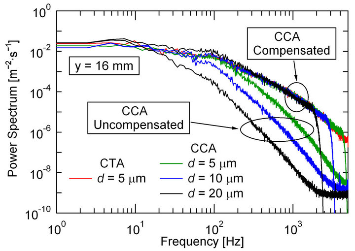
Figure 7. Power spectra of velocity fluctuations measured using three single-sensor probes driven by CCA and that by CTA at y = 16 mm where the turbulent intensities take their maxima.
μm hot-wire outputs, respectively. As seen from the above, the proposed theoretical response compensation scheme works quite well.
5.2. Adaptive Response Compensation by the Two-Sensor Technique
Before applying the two-sensor technique to the present experiment, we investigated the frequency response of the three hot-wires 5 μm, 10 μm and 20 μm in diameter to confirm that the response characteristics of these hotwires can be approximated by the first-order lag system as explained in Section 3.1. Then, we estimated the timeconstant values by the emin and Rmax methods described in Section 3.2. The results obtained at y = 16 mm are summarized in Table 2" target="_self"> Table 2. As seen from Table 2, the timeconstant values estimated by both Probe 1 and Probe 2 using the Rmax method are in good agreement with those obtained from the correlation equation proposed by Collis and Williams [17]. Figure 8 shows the compensated r.m.s. velocity distributions obtained by Probe 2 using the Rmax method (results obtained by Probe 1 is omitted due to space limitation). As seen from Figure 8, the present response compensation scheme works successfully and can provide acceptable results that are comparable to the CTA measurements, except the centerline region around y = 0 mm. This slight discrepancy near the centerline may be caused by an increase of thermal and/or fluid-dynamic interferences between the two hot-wires of the two-sensor probe shown in Figure 4.
The power spectra of both uncompensated and compensated velocity fluctuations measured at y = 16 mm are shown in Figure 9, where we also compared their distributions with those obtained by the CTA. In the present
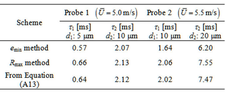
Table 2. Time-constant values estimated from emin method, Rmax method and Collis-Williams law given by Equation (A13) (y = 16 mm).
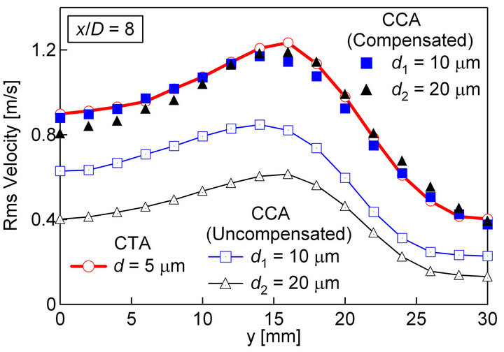
Figure 8. Rms velocities obtained by two-sensor technique using Rmax method (Probe 2).
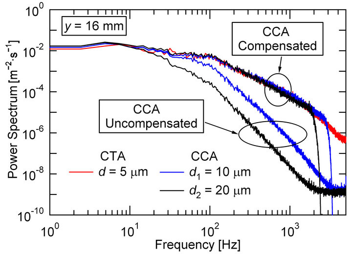
Figure 9. Comparison of power spectrum distribution using two-sensor technique using Rmax method (Probe 2).
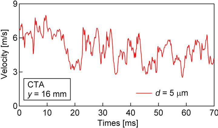
experiment, we removed high-frequency noise components in the compensated CCA outputs using a finite-impulse-response (FIR) digital filter with the cutoff frequency of 3 kHz for the 10 μm hot-wire and 2 kHz for the 20 μm one. As seen from Figure 9, the power spectra of the compensated CCA outputs agree well with the CTA result, and high-frequency velocity fluctuations up to around 2 kHz can be well reproduced. Meanwhile, Figure 10 shows a comparison of the instantaneous signal trace between the uncompensated and compensated CCA outputs measured at y = 16 mm, with a reference of the CTA output. The CTA and CCA outputs were measured independently (they are not simultaneous measurements). As seen from Figure 10(b), high-frequency velocity fluctuations have been recovered properly by the present response compensation scheme. As a result, the compensated CCA signal traces are analogous to the CTA one shown in Figure 10(a).
6. Application of Response Compensation Technique to Multi-Sensor Measurement
6.1. Multi-Sensor Probe
Multipoint measurement and analysis will help us elucidate the spatiotemporal structures of turbulent flows. Thus, in the present study, we have explored the possibilities of applying the above-mentioned response compensation scheme to the multi-sensor probe driven at the CCA mode, since the constant electric-current circuit driving the hot-wires, e.g., Figure 3(a), is much simpler and can be constructed at an even lower cost than the constant-temperature anemometer (CTA). Figure 11 shows the photographs of the multi-sensor probe constructed in our laboratory. As shown in Figure 11, sixteen tungsten hot-wires 5 μm in diameter with copper plated ends are aligned at intervals of 2 mm and soldered on steel prong tips. The configuration of the 5 μm hotwire is the same as that given in Table 1, and the entire length of the sensing part becomes 30 mm. The present
 (a)
(a)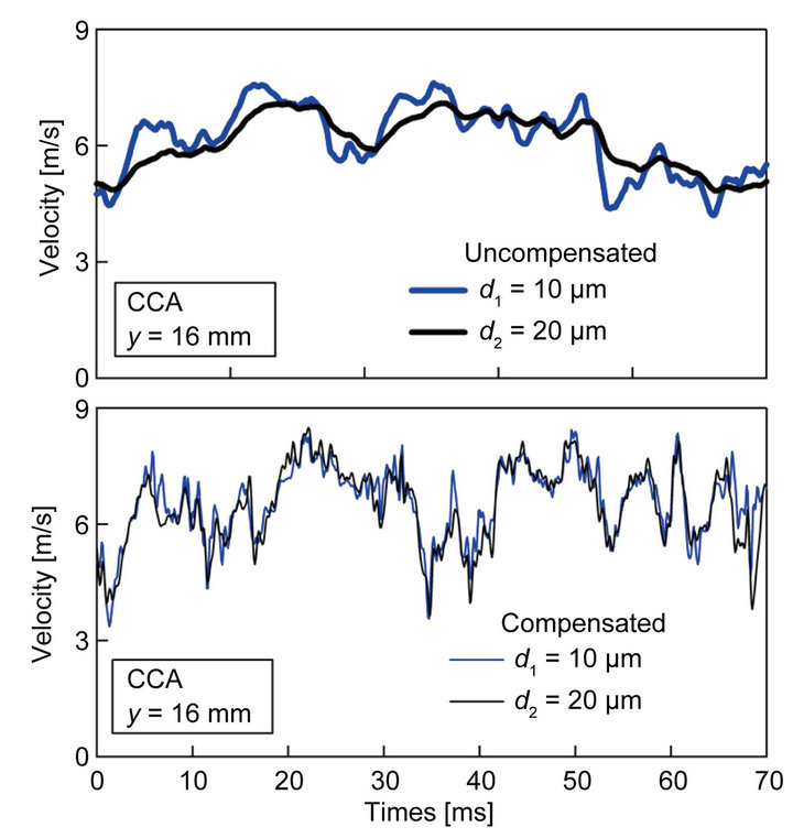 (b)
(b)
Figure 10. Instantaneous signal traces of velocity fluctuations: (a) CTA measurement by single-sensor probe; (b) CCA measurements by two-sensor probe. The CTA and CCA outputs were measured independently (they are not simultaneous measurements).
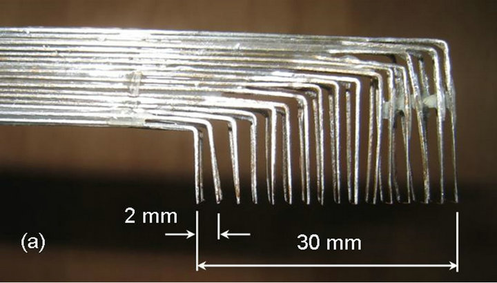
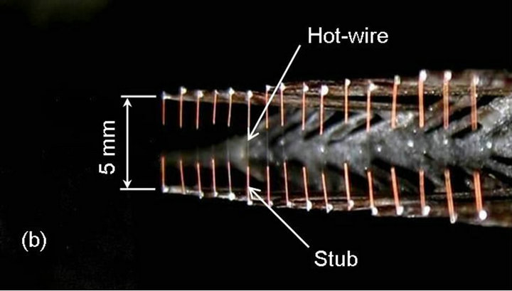
Figure 11. Multi-sensor probe consisting of sixteen 5 μm hot-wires driven at CCA mode: (a) Side view; (b) Front view.
muti-sensor probe was designed so as to measure adequately the turbulent far wake of a cylinder (Figure 4). The probe was set at the same height as the above experiment  with the probe tip positioned at y = 0 mm. When the airflow velocity at the wind-tunnel exit is 7 m/s and the probe is set at
  (cylinder diameter: D = 10 mm), the mean velocity profile in the y-direction can be sufficiently covered by the measurement range of 0 £ y £ 30 mm. We used the constant-current circuit shown in Figure 3(a) for driving the sixteen tungsten hot-wires 5 μm in diameter.
6.2. Multipoint Measurement
The multipoint measurement by the 16-channel CCA probe was performed in the turbulent far wake of the cylinder (Figure 4). Figure 5 shows the comparison between the mean velocity profile measured by the multi-sensor probe and that obtained using the single hot-wire driven by the CTA. As seen from Figure 5, the uncompensated (raw) mean velocities of the multipoint measurement are almost coincident with the CTA measurements. Naturally, as for the measurement of the mean velocity profile, the response compensation scheme need not necessarily be applied to the CCA outputs. Meanwhile, Figure 12 shows the comparison of r.m.s. velocity distributions between the multipoint measurements and the CTA result. In the present response compensation, the frequency components higher than 4.5 kHz were attenuated by a finite-impulse-response (FIR) digital lowpass filter. As seen from Figure 12, the r.m.s. velocities of the multisensor measurements compensated by using Equation (8) are in good agreement with those obtained by the CTA. Thus, a multi-sensor probe with the present response compensation scheme (Section 3.1) will work successfully to detect spatiotemporal behaviors of turbulent flow fields.
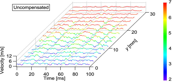
The instantaneous signal traces measured by the multisensor probe are shown in Figure 13. Figure 13(a) shows the uncompensated (raw) outputs of the 16 hot-
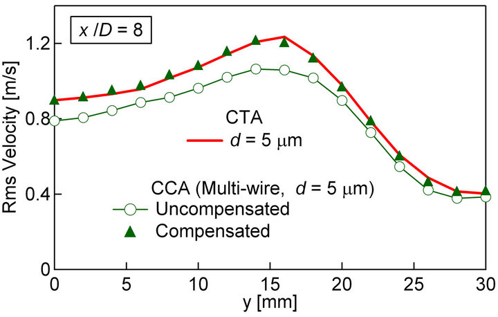
Figure 12. Comparison of Rms velocity distributions of single-sensor measurement by CTA and multipoint measurement by CCA.
 (a)
(a)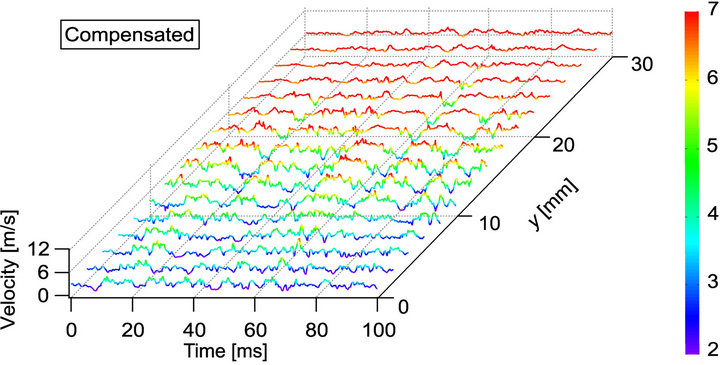 (b)
(b)
Figure 13. Instantaneous signal traces of multipoint measurement: (a) Uncompensated (raw) outputs; (b) Compensated results by theoretical response compensation scheme using Equation (8).
wires of the multi-sensor probe, in which the hot-wires are arranged at the constant intervals of 2 mm, and the cylinder was placed at y = 0 mm (see Figures 11 and 12). As seen from Figure 13(a), the mean velocity changes largely in the region of 0 £ y £ 20 mm, and the mean velocity gradient in the y direction is barely observed in the region of y ³ 20 mm. On the other hand, Figure 13(b) shows the compensated signal traces. As seen from Figure 13(b), the response compensation has reproduced high-frequency velocity fluctuations and has made it evident that large-scale fluid motions exist through the shear layer of the turbulent far wake of the cylinder. Thus, the multi-sensor probe driven by the CCA together with the digital response compensation scheme will provide a useful tool for investigating spatiotemporal structures of turbulent flows.
7. Conclusion
The constant-current hot-wire anemometer (CCA) can be realized with a very simple and low-cost electric circuit for heating the hot-wire. In the present study, we have proposed an adaptive response compensation technique to compensate for the response lag of the CCA by taking advantage of digital signal processing technology. First, we investigated the frequency response of the hot-wires 5 μm, 10 μm and 20 μm in diameter, driven by the constant-current circuit using the theoretically-derived frequency response function. Then, we developed a precise response compensation scheme based on the frequency response function of the CCA [6,7], and verified its effectiveness experimentally. Furthermore, another novel technique based on the two-sensor probe technique has been proposed, which enables in-situ estimation of the thermal time-constants of the hot-wires driven at the CCA mode to realize reliable response compensation of the CCA. To demonstrate the usefulness of the CCA, we applied the response compensation schemes to multipoint velocity measurement of the turbulent far wake of the circular cylinder by using the multi-sensor probe consisting of 16 hot-wires driven simultaneously by the very simple constant-current circuit. As a result, the proposed response compensation techniques for the CCA worked quite successfully and are capable of improving the response speed of the CCA to obtain reliable measurements comparable to those by the commercially-available constant-temperature hot-wire anemometer.
8. Acknowledgements
The authors would like to thank Dr. K. Kaifuku for his valuable assistance and advice with the theoretical response compensation scheme. This work was partially supported by a Grant-in-Aid for Scientific Research (No. 22560194) and for Young Scientists (No. 24760164) from The Japan Society for the Promotion of Science (JSPS).
REFERENCES
- J. O. Hinze, “Turbulence,” 2nd Edition, McGraw-Hill, New York, 1975.
- G. Comte-Bellot, “Hot-Wire Anemometry,” Annual Review of Fluid Mechanics, Vol. 8, 1976, pp. 209-231. doi:10.1146/annurev.fl.08.010176.001233
- G. Comte-Bellot, “Springer Handbook of Experimental Fluid Mechanics,” In: C. Tropea, A. L. Yarin and J. F. Foss, Eds., Sec 5.2.1-5.2.7, Springer, Berlin, 2007, pp. 229-283.
- A. E. Perry, “Hot-wire Anemometry,” Oxford University Press, New York, 1982.
- H. H. Bruun, “Hot-Wire Anemometry - Principles and Signal Analysis,” Oxford University Press, New York, 1995.
- K. Kaifuku, S. M. Khine, T. Houra and M. Tagawa, “Response Compensation of Constant-Current Hot-Wire Anemometer,” Proceedings of the 21st International Symposium on Transport Phenomena, Kaohsiung, 2-5 November 2010, pp. 816-822.
- K. Kaifuku, S. M. Khine, T. Houra and M. Tagawa, “Response Compensation for Constant-Current Hot-Wire Anemometry Based on Frequency Response Analysis,” Proceedings of ASME/JSME 2011, 8th Thermal Engineering Joint Conference, Honolulu, 13-17 March 2011, Article ID: T10164.
- I. Kidron, “Measurement of the Transfer Function HotWire and Hot-Film Turbulence Transducers,” IEEE Transactions on Instrumentation and Measurement, Vol. 15, No. 3, 1966, pp. 76-81. doi:10.1109/TIM.1966.4313512
- M. Tagawa and Y. Ohta, “Two-Thermocouple Probe for Fluctuating Temperature Measurement in Combustion— Rational Estimation of Mean and Fluctuating Time Constants,” Combustion and Flame, Vol. 109, No. 4, 1997, pp. 549-560. doi:10.1016/S0010-2180(97)00044-8
- M. Tagawa, T. Shimoji and Y. Ohta, “A Two-Thermocouple Technique for Estimating Thermocouple Time Constants in Flows with Combustion: In Situ Parameter Identification of a First-Order Lag System,” Review of Scientific Instruments, Vol. 69, No. 9, 1998, pp. 3370-3378. doi:10.1063/1.1149103
- R. F. Blackwelder and R. E. Kaplan, “On the Wall Structure of the Turbulent Boundary Layer,” Journal of Fluid Mechanics, Vol. 76, No. 1, 1976, pp. 89-112. doi:10.1017/S0022112076003145
- M. N. Glauser and W. K. George, “Application of Multipoint Measurements for Flow Characterization,” Experimental Thermal and Fluid Science, Vol. 5, No. 5, 1992, pp. 617-632. doi:10.1016/0894-1777(92)90018-Z
- T. Houra and Y. Nagano, “Spatio-Temporal Turbulent Structures of Thermal Boundary Layer Subjected to NonEquilibrium Adverse Pressure Gradient,” International Journal of Heat and Fluid Flow, Vol. 29, No. 3, 2008, pp. 591-601. doi:10.1016/j.ijheatfluidflow.2008.03.004
- K. Kato, K. Kaifuku and M. Tagawa, “Fluctuating Temperature Measurement by a Fine-Wire Thermocouple Probe: Influences of Physical Properties and Insulation Coating on the Frequency Response,” Measurement Science and Technology, Vol. 18, No. 3, 2007, pp. 779-789. doi:10.1088/0957-0233/18/3/030
- J. D. Li, “Dynamic Response of Constant Temperature Hot-Wire System in Turbulence Velocity Measurements,” Measurement Science and Technology, Vol. 15, No. 9, 2004, pp. 1835-1847. doi:10.1088/0957-0233/15/9/022
- A. Berson, G. Poignand and P. Blanc-Benon and G. Comte-Bellot, “Capture of Instantaneous Temperature in Oscillating Flows: Use of Constant-Voltage Anemometry to Correct the Thermal Lag of Cold Wires Operated by Constant-Current Anemometry,” Review of Scientific Instruments, Vol. 81, No. 1, 2010, Article ID: 015102. doi:10.1063/1.3274155
- D. C. Collis and M. J. Williams, “Two-Dimensional Convection from Heated Wires at Low Reynolds Numbers,” Journal of Fluid Mechanics, Vol. 6, No. 3, 1959, pp. 357- 384. doi:10.1017/S0022112059000696
- M. Tagawa, S. Nagaya and Y. Ohta, “Simultaneous Measurement of Velocity and Temperature in High-Temperature Turbulent Flows: A Combination of LDV and Three-Wire Temperature Probe,” Experiments in Fluids, Vol. 30, No. 2, 2001, pp. 143-152. doi:10.1007/s003480000149
- T. Tsuji, Y. Nagano and M. Tagawa, “Frequency Response and Instantaneous Temperature Profile of ColdWire Sensor for Fluid Temperature Fluctuation Measurements,” Experiments in Fluids, Vol. 13, 1992, pp. 171- 178. doi:10.1007/BF00218164
- M. Tagawa, K. Kato and Y. Ohta, “Response Compensation of Fine-Wire Temperature Sensor,” Review of Scientific Instruments, Vol. 76, No. 9, 2005, Article ID: 094904.
- M. Tagawa, K. Kato and Y. Ohta, “Response Compensation of Thermistors: Frequency Response and Identification of Thermal Time Constant,” Review of Scientific Instruments, Vol. 74, No. 3, 2003, pp. 1350-1358. doi:10.1063/1.1542668
Appendix A: Theoretically-Derived Frequency Response Function of the CCA
In this appendix, we have summarized the theoretical derivation processes of the frequency response function of the hot-wire probe, consisting of a fine metal wire, stub parts (copper-plated ends/silver cladding of a Wollaston wire) and prongs (wire supports) (see Figure 1).
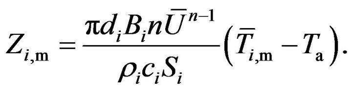
Equation (5) should be a fundamental equation for obtaining the frequency response function expressed by Equation (8). In the right-hand side of Equation (5), the term  representing the time-averaged temperature difference between the wire and surrounding fluid varies as a function of x. In the present analysis, however, we assume this term to be constant for simplicity and replace
  by the spatially-averaged temperature along the wire
 , and similarly
  by
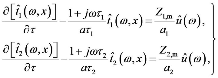
by  for the stub. As a result, the responses of the wire and stub temperatures to the velocity fluctuation u and the relevant boundary conditions are written as:
• Wire :
:
 (A1)
(A1)
• Stub :
:
 (A2)
(A2)
• Boundary conditions for Equations (A1) and (A2):
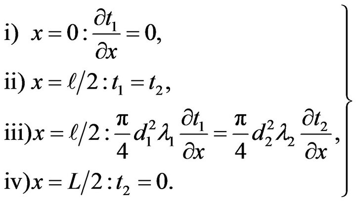 (A3)
(A3)
The boundary conditions 1) - 4) shown in Equation (A3) are formulated so as to represent the following physical requirements: 1) a temperature distribution along the heated wire is symmetrical about the origin of the x axis ; 2) at the interface
 , the temperature of the wire is equal to that of the stub; 3) heat flowing through the interface
  is assumed to be conserved; and 4) the temperature at the tip of the prong (namely, temperature of the stub at
 ) is kept at fluid temperature Ta.
In the following, we investigate theoretically the frequency response of the CCA along the lines of the procedure used in the analyses of the frequency response of a fine-wire temperature sensor [19,20] a thermistor [21]. The temperatures of the wire and the stub,  and
and , and the flow velocity
  can be written using the Fourier integrals as follows:
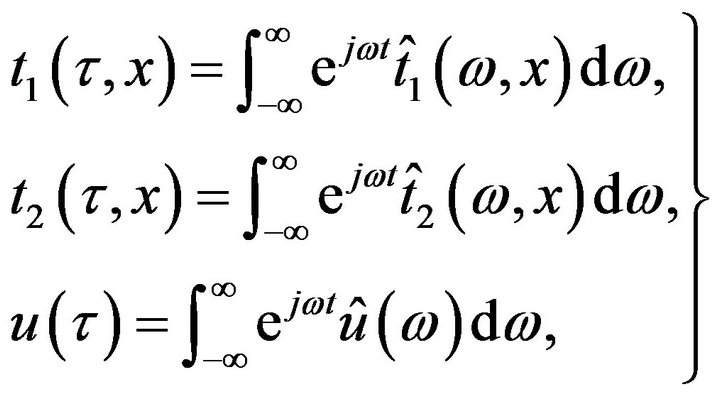 (A4)
(A4)
where j is an imaginary unit and w an angular frequency . From Eq. (A4), Equations (A1) and (A2) are transformed into the following equations:
 (A5)
(A5)
where  is represented by
 (A6)
(A6)
Equation (A5) is composed of the two differential equations on the variable (coordinate) x, and their solutions are given by
 (A7)
(A7)
where  are the undetermined coefficients, and
  is defined by
 (A8)
(A8)
The boundary conditions 1) - 4) in Equation (A3) are also written in the Fourier integrals, and are used to determine the coefficients  in Equation (A7). As a result, the frequency component of the wire temperature,
  , becomes
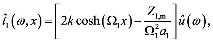 (A9)
(A9)
where k is given by
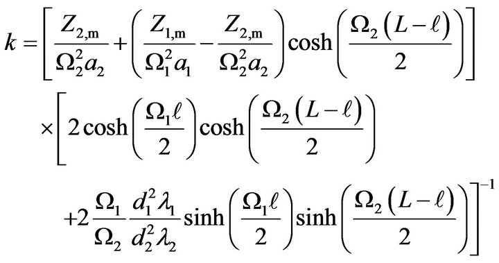 (A10)
(A10)
It is assumed that the wire temperature  can be replaced by the mean temperature
  spatially-averaged in the range of
 . Therefore, we may appraise the frequency response of the wire by averaging
  in the same range and the result
  is described as follow:
 (A11)
(A11)
From the above Equation (A11), we finally obtain the frequency response of the hot-wire probe driven by the CCA,  The result is given by Equation (8). Similarly, the frequency response of the stub
  can be obtained by determining the values of
  and
and  in Equation (A7) (not shown).
If there is no stub (i.e., ), the wire is directly connected to the prong. Equation (8) is reduced to the following simple expression:
 (A12)
(A12)
To investigate the frequency response of the CCA using Equation (8), we need to evaluate the heat transfer coefficient h that plays a key role in determining the time constants t1 and t2 as shown in Equation (6). In the present study, we use the well-known Collis-Williams correlation equation [17], which is given by
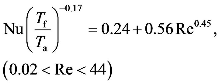 (A13)
(A13)
where Nu and Re are the Nusselt and Reynolds numbers, respectively and are defined as 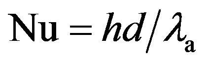 and
and 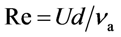 (U: flow velocity; na: kinematic viscosity of fluid); and Tf is a film temperature defined as
  (T: surface temperature of the wire). In the following, we investigate in detail the frequency response characteristics of the CCA to obtain basic knowledge of the response compensation of its output. As for the hot-wire probe to be analyzed, a fine tungsten wire 5 mm in diameter is supported by copper stubs 35 mm in diameter, and the end of the stub is connected to the prong tip.
In the present analysis, the distance between the prongs (see Figure 1), air flow velocity, fluid temperature and the electric current to drive the CCA are set to 5 mm, 4 m/s, 25˚C and 40 mA, respectively. First, we investigated the frequency response as a function of the wire length. The results are shown in Figure A1. As seen from Figure A1(a), the gain rises considerably with increasing wire length, since the heat loss due to conduction becomes increasingly dominant as the wire length decreases. Naturally, the gain becomes lowest in the case of the shortest wire. Figures A1(b) and (c) show the Bode diagram (gain and phase) of the CCA output, where the gain is normalized by the respective values at frequency f = 0 Hz. In practice, the Bode diagram shown in Figures A1(b) and (c) can facilitate the comparison of the effects of the wire length on the response of the hot-
(a)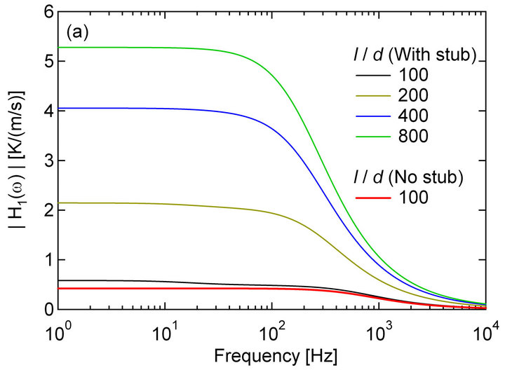 (b)
(b)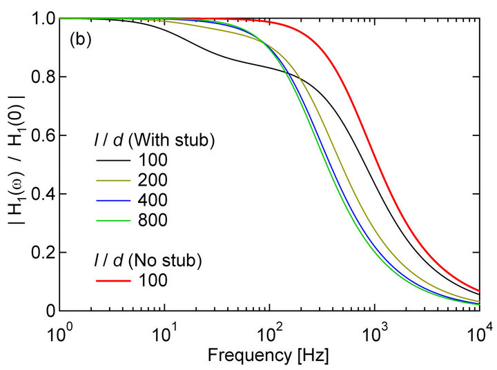 (c)
(c)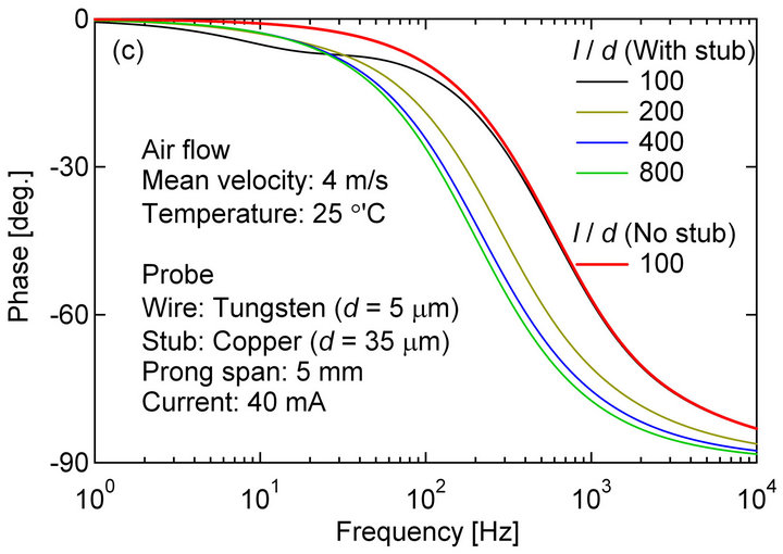
Figure A1.2. Frequency response of CCA obtained using Equation (8): (a) Absolute gain;(b) Normalized gain; (c) Phase.
wire output, and we may gain a deeper understanding of the response characteristics of the CCA. As shown in Figures A1(b) and (c), although the absolute gain attenuates considerably [Figure A1(a)], the frequency response improves in a high-frequency region over 200 Hz as the aspect ratio of the wire decreases. This is because the relative thermal inertia of the system consisting of the wire, stub and the prong diminishes with decreasing aspect ratio of the wire. On the other hand, the gain in a low-frequency region smaller than 200 Hz increases, and approaches the first-order lag system. In this first-order lag system, the gain and phase take the values of  and
and  degrees, respectively.
From these results, the no-stub case with  will give the most ideal frequency response except that the absolute gain attenuates enormously. In this contradictory situation, therefore, we must optimize the wire length by taking into account the overall signal-to-noise ratio of the measurement system used. It is noted here that being different from the CCA, the frequency response of the fine-wire temperature sensors will deviate largely from the first-order lag system even if the aspect ratio
  is greater than 400 [20].
NOTES
*Corresponding author.