ABSTRACT

Our question delves into the nature of early universe vacuum fields, and if this initial vacuum field corresponds to a configuration of early universe space-time at the start of inflation. The answer as to this came out due to wanting to know if a cosmological constant, as given in the Einstein field equations is commensurate with the byproduct of squeezed states. We compare our answer, with the influx of energy as given by a modified Heinsenberg uncertainty principle, at the start of the inflationary era. The so called influx of energy is tied into the squeezed state phenomena as written up in the onset of this article. The impetus to writing this document came from Dr. Karim, in an e mail which the author relates to, in the introduction. Our claim is that the smallness of is what is driving the existence of the squeezed states.

Keywords:

Vacuum Fields, Modified Heisenberg Uncertainty Principle, Squeezed States

1. Introduction. How to Introduce the Physics of Our Inquiry

Dr. Karim mailed the author with the following question which will be put in quotes: [1] .

The challenge of resolving the following question: At the Big Bang the only form of energy released is in the form of geometry―gravity. Intense gravity field lifts vacuum fields to positive energies. So an electromagnetic vacuum of density 10¹²² kg/m³ should collapse under its own gravity. But this does not happen―that is one reason why the cosmological constant cannot be the vacuum field. Why?

Answering this question delves into what the initial state of the universe should be, in terms of a flux of energy and space-time, and how this relates to squeezed states. To start this up, we will review first an HUP used in the initial configuration of space-time and tie it into initial squeezed states, and then from there ask about forming an initial vacuum field. Our supposition is that this vacuum field is, indeed commensurate with the initial idea of forming a cosmological “constant”. To start this off, we will introduce first the modified HUP, as formed by the author in [2] which is the influx of space-time the author then uses to create squeezed states. The work done in [2] is relevant to [3] where we look at how worm holes connect gravitational waves, as far as initial vacuum states.

Specifically, we state a new HUP formalism to come up with a change of energy expression. This change in energy will be one of the inputs into our varying over time, the cosmological constant. And the cosmological constant would be ruled out as the vacuum energy.

2. Looking at a Modified HUP, as an Energy “Driver” to the Squeezed States

We will first of all, look at the inner dynamics of the metric tensor fluctuation. To do this we encompass the following background. We will next discuss the implications of this point in the next section, of a non-zero smallest scale factor. Secondly the fact we are working with a massive graviton, as given will be given some credence as to when we obtain a lower bound, as will come up in our derivation of modification of the values [2] .

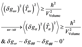(1)

The reasons for saying this set of values for the variation of the non metric will be in the 3^rd section and it is due to the smallness of the square of the scale factor in the vicinity of Planck time interval.

Begin with the starting point of [4] [5]

. (2)

We will be using the approximation given by Unruh [4] [5] , of a generalization we will write as

(3)

If we use the following, from the Roberson-Walker metric [2] .

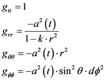(4)

Following Unruh [4] [5] , write then, an uncertainty of metric tensor as, with the following inputs

. (5)

Then, if

(6)

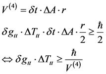
This Equation (6) is such that we can extract, up to a point the HUP principle for uncertainty in time and energy, if we use the fluid approximation of space-time [2] .

(7)

Then [2]

. (8)

Then, Equation (6) and Equation (7) and Equation (8) imply

(9)

How likely is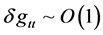? Not going to happen. The basic issue is, given as follows

(10)

Here, up to a point we are going to be writing, having, if we model the scale factor by, that

(11)

For our purposes, this corresponds to having fairly large but not infinite, but also the decisive factor in the reduction of energy density i.e. that even in the Pre Planckian regime, that the energy density be positioned for a dramatic drop in value, this so in fact that the resulting value of be very small. We will from both of these two entries obtain the following, From Equation (10) we find that if we are starting off with the dimensional scaling of [6]

(12)

which in turn may help us understand when the formation of this value occurred, i.e. [7]

. (13)

We are supposing that Equations (12), (27), (39) and Equations (13), (28), (40) holds at the formation of a Schwartzshield mass of the Universe radius. Also, here is our candidate as to the formation of an initial time step. As given.

(14)

Then, up to a point, if the above is in terms of seconds, and N sufficiently large, we could be talking about an initial non zero entropy, along the lines of the number of nucleated particles, at the start of the cosmological era. As given by making use of quantum infinite statistics as well as our adaptation of it [8] .

(15)

Initial entropy would be small, but non zero, and would be affected by strongly, i.e. the initial degrees of freedom assume would play a major role as far as how initial entropy and initial time steps would be initiated.

Therefore we have commenced setting up, from the background of the modified. HUP, modus operandi as to early universe initial conditions and the set up of what will be generic squeezing.

All this can be summed up as follows

(16)

Let us now go to the matter of what leads to squeezed states. This is extremely important.

The change in energy, as given in is enormous, i.e. almost equivalent to the entire energy budget of the Universe, at the start of the big bang, hence, to keep the minimum time step as larger than or equal to zero. How we form the change in energy will lead directly to the matter of squeezed states, which is next. i.e. what we are doing, next, is to utilize the information assumed in Equation (16), after making a detour into squeezed state formalism.

3. Background as to the Physics of What Forms Squeezed States

We are coming up with a simple scaling procedure as to link the possible changes of the cosmological “constant” with.

Secondly, we look for a way to link initial energy states, which may be pertinent to entropy, in a way which permits an increase in entropy from 10¹⁰ at the start of the big bang to about 10¹⁰⁰ today.

One such way to conflate entropy with an initial cosmological constant may be of some help, i.e. if or smaller, i.e. in between the threshold value, and the cube of Planck length, one may be able to look at coming up with an initial value for a cosmological constant as given by as given by [9] .

(17)

A way to tie in this maximum value of the vacuum energy version of the cosmological constant, in Equation (17) is to write [10] .

(18)

We submit that the essence of the squeezed state phenomena is due to the import of

(19)

i.e. the following ratio is what distinguished squeezed states from the non squeezed states

(20)

i.e. the fact we have indicates initial squeezing, of states, and I will define, here the initial vacuum energy as

. (21)

Then the maximum cosmological constant, is, instead defined by the ratio.

(22)

Our claim, is that the smallness of is what is driving the existence of the Squeezed states. We will be commenting upon this directly.

Once we get out of the regime for smallness of, we then recover having the Padmanabhan analysis of Equation (18) and approach the transition from a maximum cosmological “constant” which collapses to the regular cosmological constant, in the present era.

We will next then analyze what happens as to the situation when no longer holds. i.e..

4. Physics of When. Holds, and the Breakdown of Squeezed States

Then making the following identification of total energy with entropy via looking at models, i.e. consider Park’s model of a cosmological “constant” parameter scaled via background temperature [11] .

(23)

A linkage between energy and entropy, may be seen in the following construction, namely looking at what Kolb [12] put in, i.e.

. (24)

Here, the idea would be, possibly to make the following equivalence, namely look at,

. (25)

Note that in the case that quantum effects become highly significant, that the contribution as given by and potentially much smaller, as in the threshold of Plancks length, going down to possibly as low as 4.22419 × 10⁻¹⁰⁵ m³ = 4.22419 × 10⁻⁹⁶ cm³ leads us to conclude that even with very high temperatures, as an input into the initial entropy, that is very reasonable. We should keep in mind that we are not including in the space-time consideration of Crowell [13] in this stage of the analysis. Note though that Kolb and Turner, however, have that is at most about 120, whereas the author, in conversation with H. De La Vega, in 2009 [14] indicated that even the exotic theories of have an upper limit of about 1200, and that it is difficult to visualize what is in the initial phases of inflation. De La Vega stated in Como Italy, that he, as a conservative cosmologist, viewed defining in the initial phases of inflation as impossible [14] .

One arguably needs a different venue as to how to produce entropy initially, and the way the author intends to present entropy, initially is through initial graviton production. The question of if gravitons, especially high frequency gravitons, can be detected will compose the last part of the manuscript.

To start off with, consider what if entropy were in a near 1-1 relations with, in initially very strongly curved space time with information.

We intend to put a structure in, which may influence the evolution, and to do it in terms of known squeezed state dynamics.

5. How Squeezed State Conditions at the Onset of Inflation Affects Usual Attempts at Measurement of Coherent Relic Graviton States Due to the Smallness of

Now what could be said about forming states close to classical representations of gravitons? Venkatartnam, and Suresh, 2008 [15] built up a coherent state via use of a displacement operator, applied to a vacuum state, where is a complex number, and as annihilation, and creation operations, where one has

. (26)

However, what one sees in string theory, is a situation where a vacuum state as a template for graviton nucleation is built out of an initial vacuum state,. To do this though, as Venkatartnam, and Suresh did, involved using a squeezing operator defining via use of a squeezing parameter r as a strength of squeezing interaction term, with, and also an angle of squeezing, as used in

, where combining the

with (27) leads to a single mode squeezed coherent state, as they define it via [15] .

(27)

The right hand side. of Equation (27) given above becomes a highly non classical operator, i.e. in the limit that the super position of states occurs, there is a many particle version of a “vacuum state” which has highly non classical properties. Squeezed states, for what it is worth, are thought to occur at the onset of vacuum nucleation, but what is noted for being a super position of vacuum states, means that classical analog is extremely difficult to recover in the case of squeezing, and general non classical behavior of squeezed states. Can one, in any case, faced with do a better job of constructing coherent graviton states, in relic conditions, which may not involve squeezing?

We should note that the rest of this digression comes straight from [16] and the reader is encouraged to go to the second part of that article, and to, in fact, go to what is most relevant to the matter of our analysis, which is, as follows.

In [16] the author recites as given by Grishchkuk, [17] the existence of a representation of gravitons in the early universe. i.e. to whit, after derivations, Grishkuk, writes [16] [17]

. (28)

Then there are two possible solutions to the S.E. Grishchuk created in 1989 [17] , one a non squeezed state, and another a squeezed state. So in general we work with

. (29)

The non squeezed state has a parameter where is an initial time, for which the Hamiltonian given in Equation(30) in terms of raising/ lowering operators is “diagonal”, and then the rest of the time for, the squeezed state for is given via a parameter B for squeezing which when looking at a squeeze parameter r, for which, then instead of.

(30)

Taking Grishchuck’s formalism literally, a state for a graviton/GW is not affected by squeezing when we are looking at an initial frequency, so that initially corresponds to a non squeezed state which may have coherence, but then right afterwards, if which appears to occur whenever the time evolution,

.

A reasonable research task would be to determine, whether or not

would correspond to a vacuum state being initially formed right after the point of nucleation, with at time with an initial cosmological time some order of magnitude of a Planck interval of time seconds The next section will be to answer whether or not there could be a point of no squeezing, as Grishchuck implied, for initial times, and initial frequencies, and an immediate transition to times, and frequencies afterwards, where squeezing was mandatory. Note that in 1993, [18] Grischchuk further extended his analysis, with respect to the same point of departure, i.e. what to do with when. Having with a possible displacement operator, seems to be in common with, whereas which is highly non classical seems to be in common with a solution for which This leads us to the next section, i.e. does when of time seconds, and then what are the initial conditions for forming “frequency”?

Next, we shall attempt to understand how the frequency is set in our analysis of squeezed states, i.e. the matter of.

To do this we invoke transfer of matter-energy from a prior universe, to our present, via the use of worm holes. Hence, our open question. Before transfer from a prior universe, to our own do we have un squeezed states? i.e. can we realistically in the prior universe, contribution talk of.

i.e. this is what we are asking in the next section: Is the following true? Can we look at squeezed and unsqueezed states, analytically, while keeping the following in mind?

(31)

6. Other Models. Do Wormhole Bridges between Different Universes Allow for Initial un Squeezed States? Is the Wheeler De Witt Equation Enough, Initially to Have

This discussion is to present a not so well known but useful derivation of how instanton structure from a prior universe may be transferred from a prior to the present universe.

i.e. we look at reading off of data from the following line element [13] where we leave open the issue of if there is a change of the Cosmological constant in Equation (32) along the lines of Park [11] .

(32)

Our question is as follows. Does Equation (35) still make sense in the bridge?

Our claim, is that if there is an analytical bridge, with the:

1) The solution as taken from L. Crowell’s (2005) book [13] , and re produced here, has many similarities with the WKB method. i.e. it is semi CLASSICAL.

2) Left unsaid is what embedding structure is assumed.

3) A final exercise for the reader. Would a WKB style solution as far as transfer of “material” from a prior to a present universe constitute procedural injection of non compressed states from a prior to a present universe? Also if uncompressed, coherent states are possible, how long would they last in introduction to a new universe?

This is the Wheeler-De-Witt equation with pseudo time component added. From Crowell [13]

. (33)

This has when we do it, and frequently, so then we can consider

. (34)

In order to do this, we can write out the following for the solutions to Equation (33) above.

(35)

And

. (36)

This is where and refer to integrals of the form and. Next, we should consider whether or not the instanton so formed

is stable under evolution of space-time leading up to inflation. To model this, we use results from Crowell (2005) [13] on quantum fluctuations in space-time, which gives a model from a pseudo time component version of the Wheeler-De-Witt equation, with use of the Reinssner-Nordstrom metric to help us obtain a solution that passes through a thin shell separating two space-times. The radius of the shell separating the two space-times is of length in approximate magnitude, leading to a domination of the time component for the Reissner-Nordstrom metric

. (37)

This has:

. (38)

This assumes that the cosmological vacuum energy parameter has a temperature dependence as outlined by Park (2003) [11] , leading to

. (39)

As a wave functional solution to a Wheeler-De-Witt equation bridging two space- times, similar to two space-times with “instantaneous” transfer of thermal heat, as given by Crowell (2005) [13]

. (40)

This has as a pseudo cyclic and evolving function in terms of frequency, time, and spatial function. This also applies to the second cyclical wave function, where Equation (35) and Equation (36) Here, Equation (40) is a solution to the pseudo time WDM equation for Worm holes.

7. Further Representation of Squeezed and Unsqueezed States, Based on the Wheeler De Witt Equation for Wormholes

. (41)

This leads to the effective utilization of the issues brought up in Ref. [21] .

Now in the case of what can be done with the worm hole used by Crowell, with, if

, , , , and a kinetic ener-

gy value as given of the form. The supposition which we have the worm hole wave functional may be like, so, use the wave functional looking like where the for the Weiner-Nordstrom metric will be the same line element as Equation (32).

Note that in reviewing was given in terms of reviewing the feasibility of unsqueezed and squeezed light, and the mathematical consistency of Equation (32) as given above.

8. The Warning Given by Weiss as Far as the Limits of Relic Detection. Considerations Related by Weiss and Dr. Li as Far as Relic Detection

The main problem in these assumptions about how likely one can measure GW at all is in the assumed impossibility of measuring a “strain factor” According to Li, et al. (2009), is the sensitivity factor needed to measure GW. Weiss, in personal communications (2009) [21] states flatly in personal communications with the author that measurements of are impossible with currently achievable GW technology. To answer this, the author states that there does exist an argument by Dr. Fangyu Li’s [22] personal notes and personal communications (2009), which implies that relic GW, and by implicit assumption, gravitons, are not to be ruled out as Weiss stated was the case in personal communications with the author The assumptions the author is making is that with careful calibration, there is a way to obtain measurable relic GW, and also, possibly, graviton measurements. The author wishes to thank Professor Rainer Weiss, of MIT, in ADM 50, in November 7^th (2009) for explaining the implications of a formula for HFGW of at least 1000 Hertz for GW which is a start in the right direction i.e., a strain value of, if L is the Interferometer length, and N is the number of quanta/second at a beam splitter, and is the integration time. i.e. from Weiss, [21] the strain factor has to be given as

. (42)

For LIGO systems, and their derivatives, the usual statistics and technologies of present lasers as bench marked by available steady laser in puts appear to limit. The problem is that as Weiss explained to the author, one of the most active, and perhaps guaranteed to obtain GW sources involves the interaction of super massive black holes in the center of colliding galaxies, which would need to obtain verifiable data. Going significantly below involves an argument as given as follows: The following question was posed by a reviewer of a document given to Dr. Fangyu Li, and the author has copied his response as follows, [22] .

Quote:

“The most serious is that a background strain at 10 GHz corresponds to a (total) which violates the baryon nuclei-synthesis epoch limit for either GWs or EMWs. (Total) needs to be smaller than 10⁻⁵ otherwise the cosmological Helium/hydrogen abundance in the universe would be strongly affected...”

The answer, which the author copied from Dr. Li, i.e., from page ten of this document that if, then, is an answer to this supposition.

We reference Figure 1 in what we do below, i.e. the text of what we are referring to is linked to the curves in Figure 1.

The curve of the pre-big-bang models shows that of the relic GWs is almost constant from 10⁻¹ Hz to 10¹⁰ Hz. of the cosmic string models is about 10⁻⁸ in the region 1 Hz to 10¹⁰ Hz; its peak value region is about 10⁻⁷ - 10⁻⁶ Hz. According to more accepted by the general astro physics community values, the estimate, the upper limit of on relic GWs should be smaller than, while recent data analysis (B.P. Abbott et al., (2009)) [23] shows the upper limit of, as in figure FIX should be FIX. By using such parameters, Dr. Li estimates the spectrum FIX and the RMS amplitude. The relation between and the spectrum is often expressed as [24] L. P. Grishchuk, as

(43)

so

(44)

where, the present value of the Hubble frequency. From Equation (43), Equation (44), we have

(a) If, then

(45)

If, then

. (46)

If, then

. (47)

(b) If, then

. (48)

If, then

. (49)

If then

. (50)

Such values of would be essential to ascertain the possibility of detection of GW from relic conditions, whereas Ω_g, or in integral form

, as given by. Furthermore, one could also write for a very narrow

range of frequencies, that to first approximation, make a comparison between an integral representation of and. Note also that Dr. Li suggests, as an optimal upper frequency to investigate, then

, (51)

and

. (52)

These are upper values of the spectrum, and should be considered as preliminary. Needed in this mix of calculations would be a way to ascertain a set of input values for into?. The objective is to get a set of measurements to confirm if possible the utility of using, experimentally? FOR? The numerical count of

.

If there is roughly a 1-1 correspondence between gravitons and neutrios (highly unlikely), then

counting the number of gravitons per cell space should also consider what Buoanno wrote, for Les Houches [25] : if one looks at BBN, the following upper bound should be considered:

(53)

Here, Buoanno is using, and a reference from Kosowoky, Mack, and Kahniashhvili [26] (2002) as well as Jenet et al. (2006) [27] . Using this upper bound, if one insist upon assuming, as Buoanno (2007) does, that the frequency today depends upon the relation

. (54)

The problem in this is that the ratio, assumes that is “today’s” scale factor. In fact, using this estimate, Buoanno comes up with a peak frequency value for relic/early universe values of the electroweak era-generated GW graviton production of

(55)

By conventional cosmological theory, limits of are at the upper limit of 100 - 120, at most, according to Kolb and Turner (1991) [12] . is specified for nucleation of a bubble, as a generator of GW. Early universe models with or so are not in the realm of observational science, yet, according to Hector De La Vega (2009) in personal communications with the author,) at the Colmo, Italy astroparticle physics school, ISAPP, [13] a signal for GW and/or gravitons may be to consider how to obtain a numerical count of gravitons and/or neutrinos for

. (56)

And this leads to the question of how to account for a possible mass/information content to the graviton.

9. Conclusion. i.e. We Have Three Different Criteria as to Unsqueezed and Squeezed GW. How to Reconcile Them for Falsifiable Experimental Inquiry? What about Unsqueezed GW before the Wormhole?

The preference, the author has is to follow the convention of identifying how to solve the following limit

. (57)

The use of a modified HUP, as used by the author in [2] may in time allow for experimental investigation and vetting of the predictions given in [3] . If this is done, the author views the research endeavor as rewarding and one to be fully developed if and when possible.

We also look forward to investigating the premise of gravitational solitons brought up by [28] as well as investigation of the issues brought up by [29] - [31] . Also, what is brought up in [31] needs to be kept in mind when reviewing Equation (56) and Equation (57) above. No where do we wish to contravene the known LIGO discoveries as given in [31] .

Acknowledgements

The author thanks Dr. Raymond Weiss, of MIT as of his interaction in explaining Advanced LIGO technology for the detection of GW for frequencies beyond 1000 Hertz and technology issues with the author in ADM 50, November 7, 2009.

This work is supported in part by National Nature Science Foundation of China grant No. 11375279.

Cite this paper

Beckwith, A.W. (2016) Is the Cosmological Constant, a “Va- cuum” Field? We Explore This by Squeez- ing Early Universe “Coherent-Semi Classical States”, and Compare This to Energy from the Early Universe Heisenberg Uncertainty Principle. Journal of High Energy Physics, Gravitation and Cosmology, 2, 546-561. http://dx.doi.org/10.4236/jhepgc.2016.24047

References

- 1. Private e Mail to Beckwith, A., August 2, 2011, by Dr. Karim, M. as of 2011 Which Initiated This Paper.
- 2. Beckwith, A. (2016) Gedanken Experiment for Refining the Unruh Metric Tensor Uncertainty Principle via Schwarzschild Geometry and Planckian Space-Time with Initial Nonzero Entropy and Applying the Riemannian-Penrose Inequality and Initial Kinetic Energy for a Lower Bound to Graviton Mass (Massive Gravity). Journal of High Energy Physics, Gravitation and Cosmology, 2, 106-124.
http://dx.doi.org/10.4236/jhepgc.2016.21012 - 3. Sepehri, A. and Ali, A.F. (2016) Birth and Growth of Nonlinear Massive Gravity and It’s Transition to Nonlinear Electrodynamics in a System of Mp-Branes. http://arxiv.org/pdf/1602.06210.pdf
- 4. Unruh, W.G. (1986) Why Study Quantum Theory? Canadian Journal of Physics, 64, 128- 130.
http://dx.doi.org/10.1139/p86-019 - 5. Unruh, W.G. (1986) Erratum: Why Study Quantum Gravity? Canadian Journal of Physics, 64, 1453.
http://dx.doi.org/10.1139/p86-257 - 6. Ali, A.F. and Das, S. (2015) Cosmology from Quantum Potential. Physics Letters B, 741, 276-279.
http://dx.doi.org/10.1016/j.physletb.2014.12.057 - 7. Haranas, I. and Gkigkitzis, I. (2014) The Mass of Graviton and Its Relation to the Number of Information According to the Holographic Principle. International Scholarly Research Notices, 2014, Article ID: 718251. http://www.hindawi.com/journals/isrn/2014/718251/
- 8. Ng, Y.J. (2008) Spacetime Foam: From Entropy and Holography to Infinite Statistics and Nonlocality. Entropy, 10, 441-461. http://dx.doi.org/10.3390/e10040441
- 9. Beckwith, A.W. (2008) Symmetries in Evolving Space-Time and Their Connection to High- Frequency Gravity Wave Production. AIP Conference Proceedings, 969, 1018-1026.
arXiv: 0804.0196 [physics.gen-ph]. - 10. Padmanabhan, T. http://ned.ipac.caltech.edu/level5/Sept02/Padmanabhan/Pad1_2.html
- 11. Park, D.K., Kim, H. and Tamarayan, S. (2002) Nonvanishing Cosmological Constant of Flat Universe in Brane-World Scenario. Physics Letters B, 535, 5-10.
http://dx.doi.org/10.1016/S0370-2693(02)01729-X - 12. Kolb, E. and Turner M. (1994) The Early Universe. Westview Press, Boston.
- 13. Crowell, L. (2005) Quantum Fluctuations of Space-Time. Vol. 25, World Scientific Series in Contemporary Chemical Physics, Singapore.
- 14. De La Vega, H. (2009) Lecture on Cosmology, and Cosmological Evolution, as Given as a Lecture at the ISAPP (International School of Astro Particle Physics). Cosmic Microwave Background and Fundamental Interaction Physics, Como, 8-16 July 2009. (Personal Observations Given to Author)
- 15. Venkatartnam, K.K. and Suresh, P.K. (2008) Density Fluctuations in the Oscillatory Phase of Nonclassical Inflaton in FRW Universe. International Journal of Modern Physics D, 17, 1991-2005.
http://dx.doi.org/10.1142/S0218271808013662 - 16. Beckwith, A. (2011) Detailing Coherent, Minimum Uncertainty States of Gravitons, as Semi Classical Components of Gravity Waves, and How Squeezed States Affect Upper Limits to Graviton Mass. Journal of Modern Physics, 2, 730-751. http://dx.doi.org/10.4236/jmp.2011.27086
- 17. Grishchuk, L. and Sidorov, Y. (1989) On the Quantum State of Relic Gravitons. Classical and Quantum Gravity, 6, L161-L165. http://dx.doi.org/10.1088/0264-9381/6/9/002
- 18. Grishchuk, L. (1993) Quantum Effects in Cosmology. Classical and Quantum Gravity, 10, 2449-2478.
http://dx.doi.org/10.1088/0264-9381/10/12/006 - 19. Martín-Moruno, P. and González-Díaz, P.F. (2009) Thermal Radiation from Lorentzian Wormholes. Physical Review D, 80, 024007. http://dx.doi.org/10.1103/PhysRevD.80.024007
- 20. Garay, L.J. (1991) Quantum State of Wormholes and Path Integral. Physical Review D: Particles and Fields, 44, 1059-1066. http://dx.doi.org/10.1103/PhysRevD.44.1059
- 21. Weiss, R. (2009) Private Discussions with the Author, at ADM 50, Fall 2009, in Texas A and M University.
- 22. Li, F. (2009) Personal Communication with the Author in Chongqing University, November, 2009.
- 23. Abbott, et al. (2009) An Upper Limit on the Stochastic Gravitational-Wave Background of Cosmological Origin. Nature, 460, 990-994. http://dx.doi.org/10.1038/nature08278
- 24. Grishchuk (2001) Relic Gravitational Waves and Their Detection. In: Lämmerzahl, C., Everitt, C.W.F. and Hehl, F.W., Eds., Gyros, Clocks, Interferometers...: Testing Relativistic Gravity in Space, 562, 167-192. http://dx.doi.org/10.1007/3-540-40988-2_9
- 25. Buonanno, A. (2007) Gravitational Waves. https://arxiv.org/abs/0709.4682
- 26. Kosowoky, A., Mack, A. and Kahniashhvili T. (2002) Gravitational Radiation from Cosmological Turbulence. Physical Review D, 66, 024030. http://dx.doi.org/10.1103/PhysRevD.66.024030
- 27. Jenet, F., et al. (2006) Upper Bounds on the Low-Frequency Stochastic Gravitational Wave Background from Pulsar Timing Observations: Current Limits and Future Prospects. The Astrophysical Journal, 653, 1571. http://dx.doi.org/10.1086/508702
- 28. Belunski and Verdaguer (2001) Gravitational Solitons. Cambridge University Press, Cambridge.
- 29. Corda, C. (2009) Interferometric Detection of Gravitational Waves: The Definitive Test for General Relativity. International Journal of Modern Physics D, 18, 2275-2282.
http://arxiv.org/abs/0905.2502
http://dx.doi.org/10.1142/S0218271809015904 - 30. Corda, C. (2007) A Longitudinal Component in Massive Gravitational Waves Arising from a Bimetric Theory of Gravity. Astroparticle Physics, 28, 247-250.
http://arxiv.org/abs/0811.0985
http://dx.doi.org/10.1016/j.astropartphys.2007.05.009 - 31. Abbott, B.P., et al. (LIGO Scientific Collaboration and Virgo Collaboration) (2016) Observation of Gravitational Waves from a Binary Black Hole Merger. Physical Review Letters, 116, Article ID: 061102. https://physics.aps.org/featured-article-pdf/10.1103/PhysRevLett.116.061102