Open Journal of Modern Hydrology
Vol.3 No.4(2013), Article ID:38961,16 pages DOI:10.4236/ojmh.2013.34029
Remote Monitoring of Vegetation Managed for Dust Control on the Dry Owens Lakebed, California
![]()
HydroBio Advanced Remote Sensing, Santa Fe, USA.
Email: david@hydrobioars.com
Copyright © 2013 David P. Groeneveld, David D. Barz. This is an open access article distributed under the Creative Commons Attribution License, which permits unrestricted use, distribution, and reproduction in any medium, provided the original work is properly cited.
Received September 10th, 2013; revised October 10th, 2013; accepted October 18th, 2013
Keywords: Dust Control; Remote Sensing; Monitoring; Managed Vegetation; NDVI; Owens Lake; California
ABSTRACT
A monitoring program was developed to assess the cover of saltgrass managed for dust control on the saline dry Owens Lake. Although the original intent was to manage the vegetation as total cover that included green and senesced leaf and stem material, aged leaves that make up a large proportion of total cover were not differentiable spectrally from the background salt and lakebed. Hence, greenness-based indices were explored for detection of plant recruitment. Since all plant cover begins as green and growing, greenness indices provide a measure of all future cover whether living or senesced. The criteria for judging compliance were changed so that spatially variable vegetation cover measured as a milestone will need to be met in the future. A derivative of NDVI, NDVIx, calculated using scene statistics, proved highly accurate, to about 0.001 of this index and with an average signal to noise ratio of 64. This high level of accuracy allowed detection of small changes in vegetation growth and vigor. Performance according to the benchmark-as-par standard was determined through combined use of cumulative distribution functions and derivative maps.
1. Introduction
Prior to dust control efforts that began during the first decade of this millennium, the Owens Dry Lake, located in Eastern Central California (Figure 1) was the single largest source of anthropogenic PM10 in the western hemisphere (GBUAPCD 2003). PM10 is particulate matter less than 10 μm in aerodynamic diameter that has been implicated in reducing respiratory health [1]. This dust was caused by hydrologic changes due to diversion of water from the 280 km2 lake.
The Owens River that supplies water to the Owens Lake was diverted nearly entirely to the City of Los Angeles beginning in 1913. Prior to diversion, Owens Dry Lake was filled with water but was declining due to irrigation diversion. The lake desiccated completely by 1927 after complete diversion to Los Angeles [2].
Owens Lake has been the terminus for Owens River during the past several thousand years, concentrating the salts received from regional runoff [3,4], and hence, was highly saline before desiccation. Salts stranded in the lakebed are a causal factor for dust releases from the surface due to temperature-controlled salt crystal precipitation that destroys soil cohesion and permits winds of only 7.5 m/s (15 kts) to ablate the dusty surface [5]. Large scale dust releases occur during the winter, generally starting about October 1 and lasting until the end of June, a period recognized as the dust season by the Great Basin Unified Air Pollution Control District (District) whose responsibility it is to monitor and enforce regional air quality.
According to the State Implementation Plan (SIP) required by California state law, SB270, Owens Lake dust control is mandated for the Los Angeles Department of Water and Power (Department) that exports the water [6]. The District is the authority for ensuring compliance and has identified three dust control measures that provide some form of surface cover: gravel, vegetation, or shallow flooding. The Department has opted to apply shallow flooding nearly exclusively, while developing approximately 912 ha (2239 ac) of saltgrass (Distichlis spicata L.), known as the Managed Vegetation Area (MVA) (Figure 1). Saltgrass forms an effective dust control measure on the MVA because its canopy creates aerodynamic roughness that reduces or eliminates erosive wind energy. The vegetation’s rhizomatous root system also holds the soil in
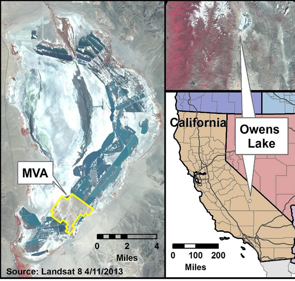
Figure 1. Location map for the Owens Lake and the MVA.
place.
This paper describes development and application of an operational remote sensing program to evaluate MVA vegetation. A second purpose is to provide guidance for those interested in generation of highly accurate vegetation indices appropriate for evaluating vegetation performance through time. A third purpose is to provide a description of the MVA program and the complexities for monitoring in case a similar program is ever contemplated at another location.
1.1. Description of the Managed Vegetation Area
The location of the MVA was formerly one of the most productive PM10 sources on the lakebed primarily because mesoscale topographic influences force winds generated during winter frontal passage into a strong northsouth trend, often impinging upon this region of the lakebed (Figure 2). The MVA soils consist of clay to sand sized particles with the sand having been moved and concentrated by aeolian processes [7].
The Owens Lake environment is highly arid with annual average precipitation less than nine centimeters per year [8]. Supplementary irrigation is necessary to supply the planted vegetation and to leach salts from the highly saline lakebed. The site was prepared by constructing a series of north-south trending rows separated by furrows spaced 1.5 m (5 ft) apart. A single drip irrigation tube was placed along the center of each row to provide leaching to move salts downward from each row crown. Preparation of the MVA site required over 5000 km of drip irrigation tubing to serve the row tops, alone.
For planting the saltgrass (Distichlis spicata, L.), accessions were collected from around the lake, cultivated
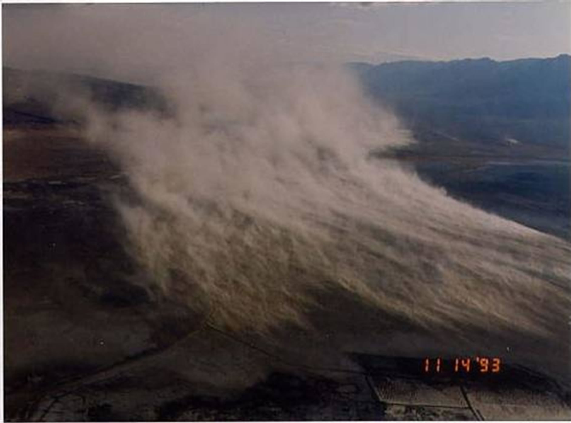
Figure 2. Dust storm from a strong northerly wind across the location of the MVA nine years before construction. The width of the dust plume is about 2 km.
separately, and then planted as plugs. Spaced every 0.3 m, this required over 17 million separate saltgrass plugs, each planted by hand. The saltgrass cover is irrigated with a blend of brine drained from the site and fresh water diverted from the Los Angeles Aqueduct that is acidified with dilute sulfuric acid to alleviate salt precipitation within the drip irrigation emitters and tubing. The plantings were made in blocks of 16.2 hectares (40 acres) separated by roadways (Figure 3). A system of French drains was established that run either parallel, or at 45 and 90 degree angles to the alignment of the planted rows. Associated pumps and piping operate this infrastructure.
Remote sensing is required to evaluate the vegetation across the large area of the MVA. Vegetation cover varies spatially and so must be assessed spatially because some areas are problematic for establishing and growing saltgrass, while other locations may foster heavy vegetation cover (Figure 3). Accurate monitoring also provides advance indications of trends in growth or decline, thus allowing proactive changes in management to avoid loss of cover that could eventually compromise air quality. Because of the scale of the MVA, earth observation satellite data (EOS; e.g., Landsat TM, Quickbird, SPOT, etc.) are required to make the evaluation.
1.2. Criterion for Judging MVA Compliance
The 2003 SIP required that each 0.405 ha (1.0 acre) of the MVA contain at least 50% cover by vegetation for dust control [6]. The MVA was planted in 2002 and during the next five years it became apparent that vegetation growth on portions lagged severely from impaired drainage and concentration of salts due to evapotranspiration of the brine irrigation (Figure 3). These constraints prevented meeting the SIP criterion for 50% total cover on all areas.
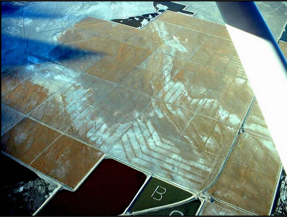
Figure 3. Oblique wintertime air photograph of the MVA showing vegetated blocks and roadways. Extensive lightcolored patterns have poor drainage, shallow groundwater, and are salt affected. This pattern is crossed with darker vegetated lines (some at 45˚ angles) that overlie drains.
No significant areas of blowing dust occurred within the MVA during the initial five years and so the vegetation cover criteria were adjusted at the discretion of the District’s Air Pollution Control Officer. The MVA vegetation cover, though poorly established in some areas, provided adequate protection from wind erosion and so a new criterion for vegetation cover was adopted to achieve existing or better cover on all areas. The new criterion recognized the stabilizing effect of the established cover while allowing low or non-emissive areas of poor cover to be accepted. This yardstick must be applied spatially, since concentration of low cover in one portion of the MVA could well lead to emissions. This low cover was set equal to the spatially-discrete peak annual cover that was measured on October 4, 2007 using a TM5 image. This spatial limit to be equaled or exceeded will be called “par”, meaning a minimum condition to be met. Application of par requires determination whether peak green growth during a subsequent year attained parity with the 2007 baseline.
The replacement criterion for achieving par vegetation growth was an important change that enabled accurate remote sensing of the MVA vegetation.
1.3. Spectral Properties and Detection of Vegetation Cover
As the MVA saltgrass grew and matured, different remote sensing methods were required to estimate cover. All initial methods used regression of remotely-sensed indices against ground truth cover that was estimated by point frequency frame [9]. The point frequency frame provides an estimate of ground cover through tallies of the first contact of vegetation by the tips of pins that are manually passed vertically downward, while the observer carefully judges the first contact of each point with leaves, stems or flowers of the vegetation. The pins are mounted in a frame and have sharpened tips for exact judgment of contacts. Sharpening the pins is important because the pin tip must be regarded as dimensionless. The total number of contacts divided by the total number of pins is an accurate estimate of fractional plant cover. Because it is labor intensive, point frequency measurements are not appropriate for monitoring at the scale of the MVA, but only for calibration of remotely-sensed data.
When the saltgrass plugs were establishing during the first season, the canopy consisted solely of green plant material and this enabled use of the normalized difference vegetation index, NDVI, that was calibrated to groundtruth supplied by point frame measurements of total cover made at discrete points across the site. During the second season and for the next two years, the ground cover matured and senesced each year, adding a thatch of dead material that contributed cover toward the goal of 50% cover that was required by the SIP. When senesced vegetation constituted the majority of cover, NDVI could no longer be used to evaluate total cover because the majority of the canopy consisted of non-green material that produced little NDVI response. This was solved by adoption of an index formed by the ratio of near infrared (NIR)/Green (Landsat TM and Quickbird bands 4/2) that was initially relatively accurate for evaluating total senesced cover (regression r2 = 94%). This index was applied in early winter after the saltgrass canopy had completely senesced but before loss of leaves through wind action or flattening of the canopy due to rare winter snow loads.
After 2005, senesced vegetation indices were no longer accurate due to a progression in coloration for aging canopy cover: 1) first as green, living material; 2) as yellowing leaves during tissue dieback; 3) as a golden orange during the first and second seasons of senescence; and finally 4) as a silver color due to weathering. In a spectrometry study using a FieldSpec Pro™, the data were converted into Landsat ETM7+ equivalent spectra using published band sensitivities. As shown in Figure 4, the last stage, silver, was found to be indistinguishable from bare substrate because ratios of the various bands could not be used to develop an index that would distinguish plant material from the background soil and saltcrust. Hence, total cover containing silver cannot be detected using EOS remote sensing. Locations were observed on the MVA to have silver material that occupied up to 90% of the total canopy cover.
Changing the initial SIP goal from 50% total cover to a spatially-discrete par approach enabled a new and accurate monitoring method that evaluated green living cover. Back-comparison of green cover from the previous growing season provides a simple assessment for whether the
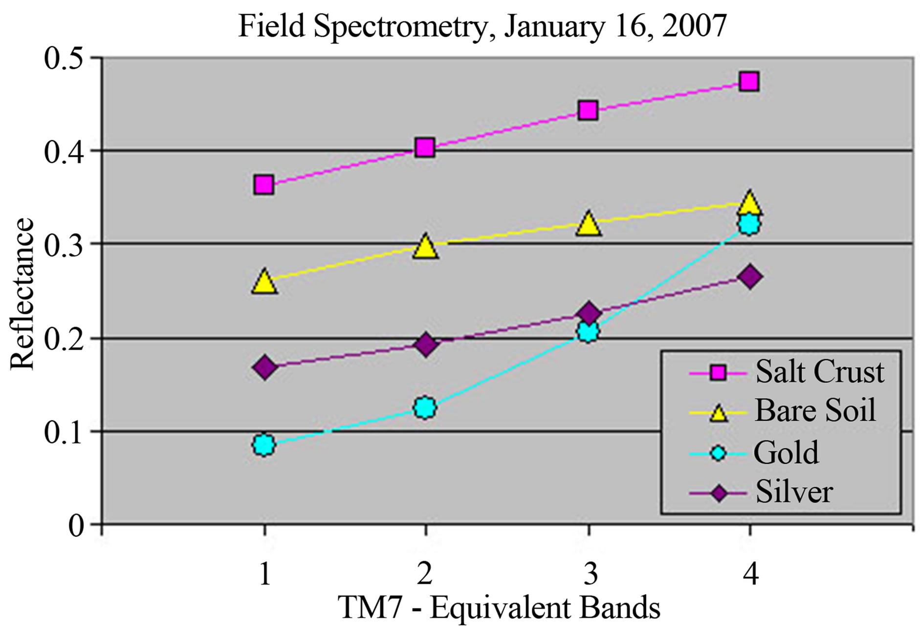
Figure 4. Aged and senesced saltgrass attains a silver color with the same ratiometry as in all bands and cannot be distinguished from bare soil or salt crust.
measured value attained par, or not. The changed criterion enabled the operational remotely-sensed monitoring system described in this paper.
Green, living cover can be measured with self-calibrated indices that have been shown to be highly accurate and useful for analysis of plant ecohydrology [10-12]. Such indices have potential for high levels of accuracy on the MVA because the vegetation is a monoculture of one species, saltgrass. During the growing season active living tissues are green, and therefore detectable with such indices.
1.4. Maintaining the Integrity of the Specifications
High levels of accuracy and measurement robustness are desired features for a competent vegetation monitoring program. Initially, the 2003 SIP required use of point frame measurements for linear regression calibration of indices using EOS data [6]. The accuracy and robustness of the point frame for measuring green living cover is important because of the spectral limitations for detection of total cover. Groundtruth using the point frame method, plus regression, were evaluated against the use of an EOS vegetation index calibrated using only scene statistics. For this comparison, a study was undertaken to understand the limitations of the point frame method.
To assess potential error, point frequency data were collected using two separate methods, each employed by the Department and the District during June 13-15, 2007. The measurements were made on a range of 14 carefully chosen sites with homogeneous cover and canopy colors. The timing of the measurement, early in the growing season, enabled separate point frame evaluation of all colors of the saltgrass canopies.
The District gathered point frame data manually using a metal frame that held a rack of 14 pins. The frame was deployed at 28 locations selected to evenly sample within a 5 m radius circle surrounding a central marking stake. The Department used a photographic method, whereby eight nadir-look photos were located according to a set scheme that was deployed around the center stake. These photos were taken to the office and displayed with a grid overlay for judging the grid contacts with vegetation—a direct analog of the manual method. The color of the contacted plant material was recorded for both methods.
A comparison of total vegetation cover for point frame and digital point frame methods showed excellent agreement (r2 = 0.979) (Figure 5). These differences were minor compared to the distribution of the two data sets when evaluating constituent canopy colors of green, gold and silver. While the percent silver and gold cover were moderately well correlated (r2 values of 0.877 and 0.817, respectively) green cover measurements were rather weakly correlated (r2 of 0.662; Figure 5). Given the high correlation for total cover, the lack of agreement between the two data sets was due, mostly, to the subjectivity in deciding canopy color. Large errors introduced by subjective color judgment during point frequency data acquisition necessarily reduces accuracy of the resulting classification of vegetation cover using EOS data.
Rather than making subjective dichotomous decisions for what is green in canopies containing gradations, such gradations are well captured by EOS data, alone. Thus, using point frame data to calibrate images was bypassed in favor of calibration of EOS data using scene statistics.
2. Methods Chosen for Processing EOS Data
An EOS index, NDVIoffset first described by Baugh and Groeneveld [10] was selected as the basis for monitoring vegetation on the managed vegetation area. NDVIoffset is derived from normalized difference vegetation index (NDVI) by subtracting an offset value determined from
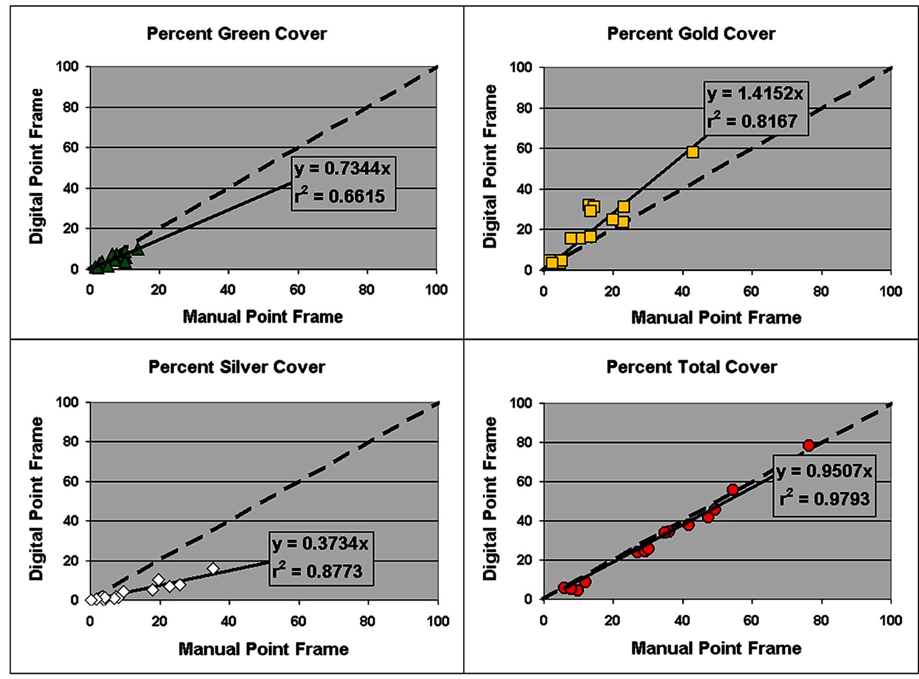
Figure 5. Comparison of percent cover green, gold and silver material measured at 14 sites by manual and digital point frame.
scene statistics. NDVIoffset was shown to yield results superior to NDVI and nearly all other indices in prediction of a known linear relationship for promotion of vegetation growth by antecedent precipitation [6]. The generation of NDVIoffset corrects for the effects of attenuation and scattering from atmospheric aerosols and for soil background coloration in a single operation.
Peak season green vegetation growth is the target for analysis of MVA performance since this is the greatest expression of plant cover recruitment that maintains surface stability for dust control. For the persistent leaves of saltgrass plants receiving repeated irrigation through the growing season, peak expression has occurred most commonly in early fall. Table 1 provides the dates and the EOS platforms that were used, all generated by the Landsat program.
A late season image may not always capture the peak of the green growth expression. Therefore, in addition to evaluating late season images, to confirm that the peak conditions have been recorded and that the image is not unduly affected by atmospheric aerosols, it is advisable to evaluate images through the entire growing season for confirmation. The vegetation captured in an annual series of images should increment through the season in a rational fashion, growing or declining smoothly through the season, rather than showing high-low fluctuations. Cumulative distribution functions (CDFs) displaying the cumulative pixel counts on the y axis and the NDVI derivative on the x, were used to compare the imagery through the growing season. In all cases, the annual image series yielded gradually changing vegetation cover through the season, taken to indicate that processing was correct and that the peak season image was acceptable.
2.1. EOS Imagery
Although any of the EOS platforms that supply red and near infrared bands could be used for a program to detect the green cover at the MVA, Landsat TM data were used for development because they were made available free of charge through http://glovis.usgs.gov/.
Six years of imagery were chosen for the comparison (Table 1). Landsat TM5 images were selected to represent 2007 through 2011 and in 2012, this EOS platform ceased operation. Landsat ETM7+ data were selected for 2012, however, these data are flawed due to stripes of missing data. The missing data stripes caused an average loss of coverage of only about 5.2% of the MVA, and so,
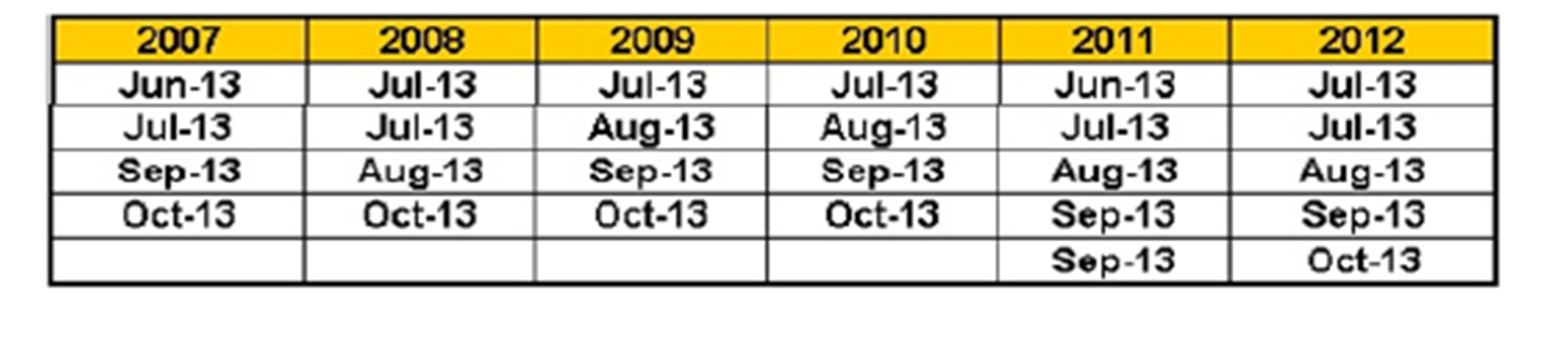
Table 1. Images chosen for analysis of trend. All images were Landsat TM5 except 2012 that were Landsat ETM7.
do not greatly affecting the quality of the comparison. The MVA is located near the center of the overall ETM7+ scene in a location where the missing data constitute only small areas with mixes of high and low vegetation cover—omissions were judged to not induce bias. For comparison of CDFs, the pixel counts for the 2012 scenes were adjusted to be equivalent to other years.
2.2. Image Processing
Calculation of top of atmosphere reflectance for Landsat data products followed methods outlined in the Landsat 7 Data User’s Handbook [13]. Following image processing, all images were geocorrected to a high resolution Quickbird panchromatic base image (0.6 m pixels) that was previously corrected to a net of carefully surveyed ground targets.
Following geocorrection, a 0.405 ha grid file was applied to mask out roads and edges from consideration in the statistical examination (Figure 6). Masking removed any potential gridcell that could possibly contain edge pixel contamination. Inclusion of edge pixels was judged to be a significant problem since unvegetated pixels among images would cause grid cell values to fluctuate according to the variable amount of unvegetated roadway that could be covered. Grid cells that could contain edge pixels were eliminated if a portion of at least one roadway or boundary pixel fell within a pixel hypotenuse (42.4 m).
2.3. Calculating NDVI and NDVIoffset
NDVI, the first step in creation of the derivative indices
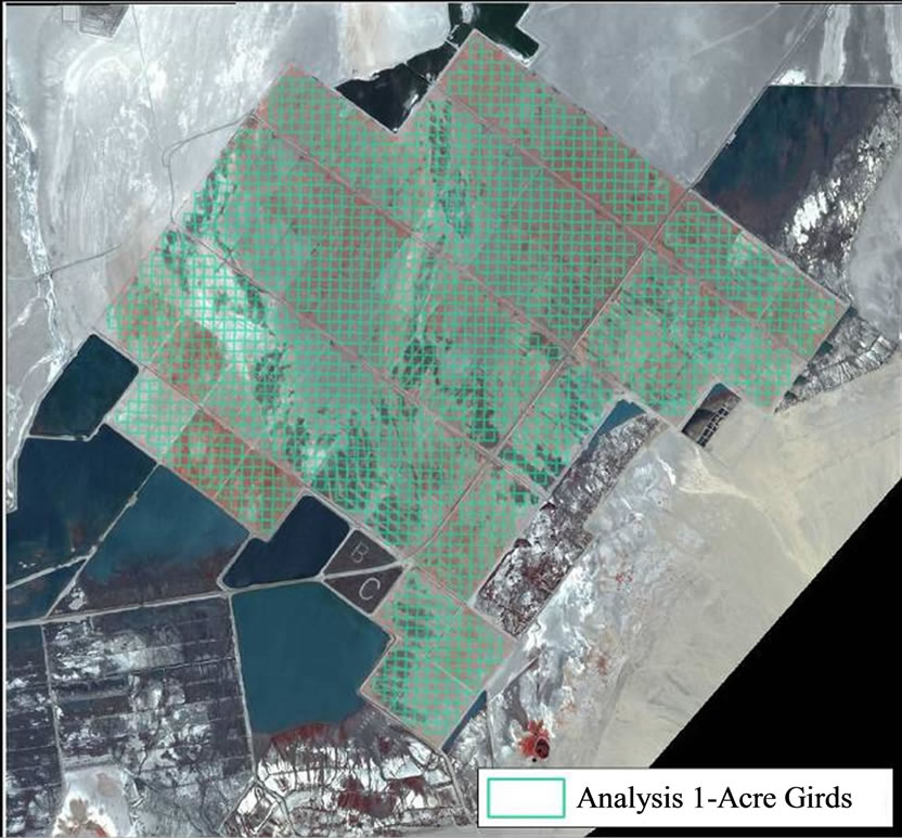
Figure 6. Grid cells (0.405 ha) that are used twice in the data processing—first to clip edge pixels and roadways and after statistical analysis and further processing, to sort the data into the grids for comparison of performance over time.
that are used for change assessment, was calculated from red and NIR TM data according to Equation (1), appropriate for the ith pixel:
 (1)
(1)
NDVIoffset is a simple shift of the NDVI distribution leftward so that zero vegetation cover approximates the soil background. To calculate NDVIoffset the raw NDVI data are displayed as a CDF such as that shown in Figure 7. The amount of the shift is determined from linear regression calculations on the lowest, near-linear limb of the NDVI CDF the x-intercept of the regression line, NDVI0 and is termed NDVI0, approximating the soil background NDVI value [10]. For the ith pixel:
 (2)
(2)
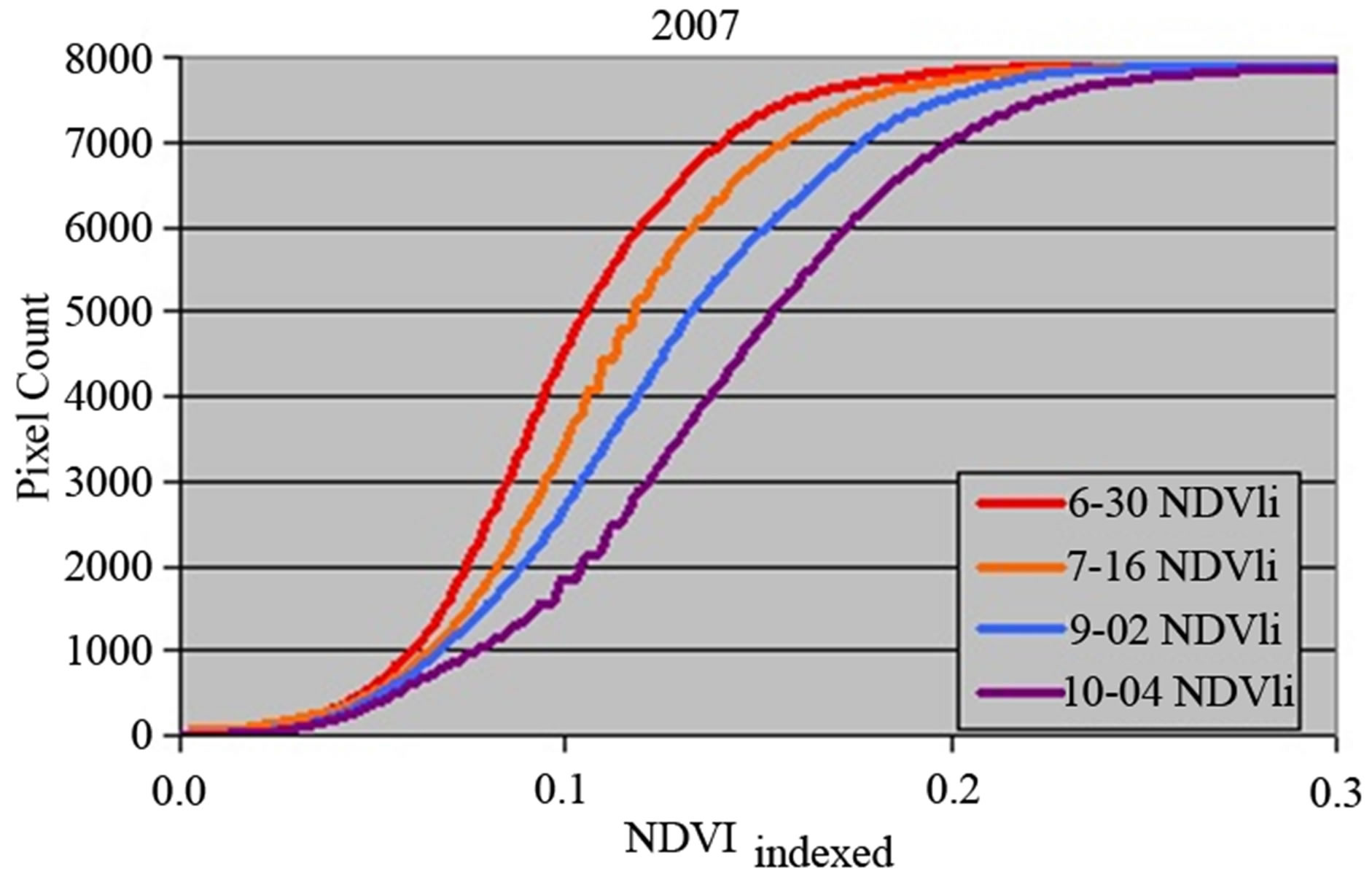
The regression interval chosen for calculating NDVI0 is best established after study of a number of images. The lower CDF region contains decreasing expression of the green canopy over a background of non-green mixed cover of soil and senesced vegetation canopies. To use Landsat TM data, it is necessary to examine the CDF to check that the interval does not contain waviness as is visible in Figure 8, due to low bit precision (Landsat TM5 data are 8 bit). If so, the interval must be expanded to bridge across the wavy region to emulate the result that would occur were the CDF smooth. The CDF interval chosen for fitting the regression relationships in Figure 8 was from 500 to 1000 pixels, constituting an interval of between six and 13 percent of the approximate total 7900-pixel distribution (software derived pixel counts may vary).
The regression of pixel intervals chosen on the CDF is solved for y = 0, and this yields an x intercept, NDVI0, that is then subtracted from all NDVI values to shift the NDVI curve leftward (Figure 9). This method provides an unbiased estimate of a point of near-zero vegetation,
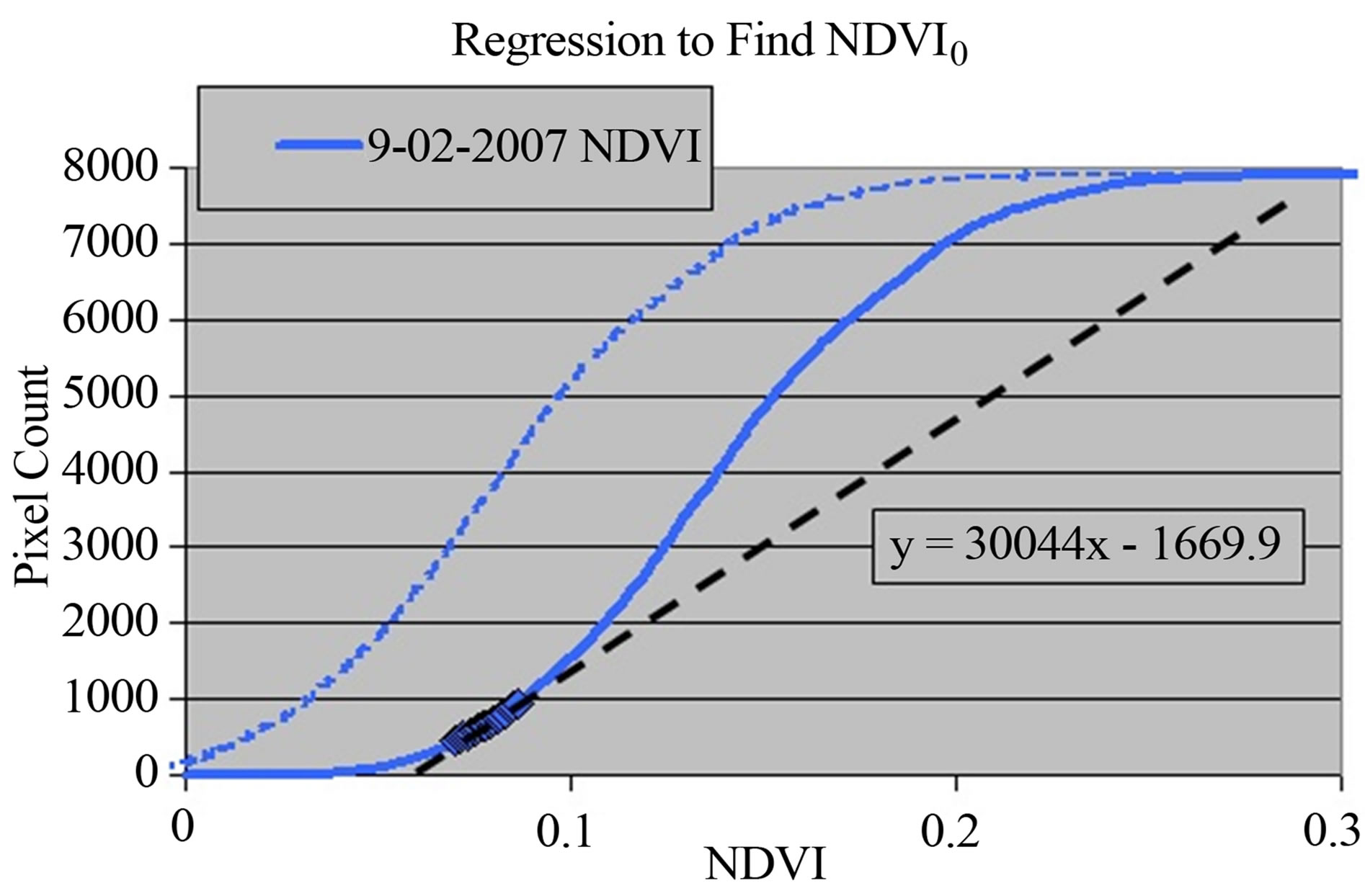
Figure 7. NDVI0, the x-intercept for the regression of the selected points, is the solution y = 0. NDVI0 is subtracted from all NDVI values to shift the distribution to the left, yielding NDVIoffset (dotted blue).
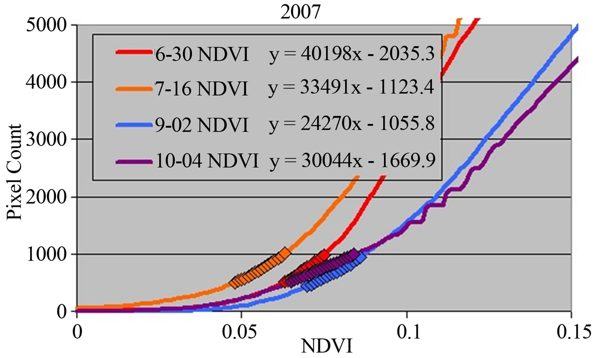
Figure 8. Four NDVI CDFs from 2007 with points chosen for regression. The regression equations were solved for y = 0 to find the x-intercepts of the curves (NDVI0). Waviness in the region of 0.10 to 0.13 NDVI for the October image is a factor of bit precision.
NDVI0, and removes most of the effects of atmospheric scatter and attenuation and is effectively a statisticallyderived estimate of the value for bare soil. Equation (2) collects the CDF curves together so that they increment correctly with increasing green expression as the season progresses. As the canopy becomes more and more green, the curves push rightward, In Figure 9 the rightward push of the increasing greenness culminates with the October image that generally captured the season peak.
The calculation of NDVIoffset provides results that are reproducible and consistent, confirming that the calculation of NDVIoffset corrects the vegetation signal relationally. NDVIoffset is only a first order estimate of bare soil that places the images in correct relation. A second step, indexing to NDVIx, was necessary to further calibrate the images for comparison to the October 4, 2007 benchmark. As shown in Figure 9, NDVIx solves a problem of truncation that occurs at the lowest levels of plant cover.
2.4. Calculating NDVIX
In the middle graph of Figure 9, NDVIoffset truncates the vegetation distribution values below zero that still may be slightly vegetated. If zero NDVIoffset is logically used for the threshold for evaluating MVA vegetation performance, there will be many pixels that are excluded and whose progress cannot be tracked. Since the analysis of vegetation performance for the MVA is made for each grid cell, pixels assigned a zero value also skew grid cell averages for spatial assessments and induce greater variability in the grid cell values that have poor cover. To overcome this problem an additional step was devised, indexing, that corrects all CDF’s to be relative to a benchmark image. For the MVA, this benchmark image is the October 4, 2007 to which all other images are compared.
A standard bare ground NDVI value for the 2007
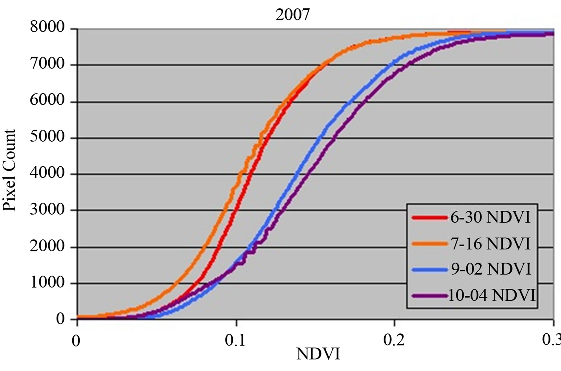
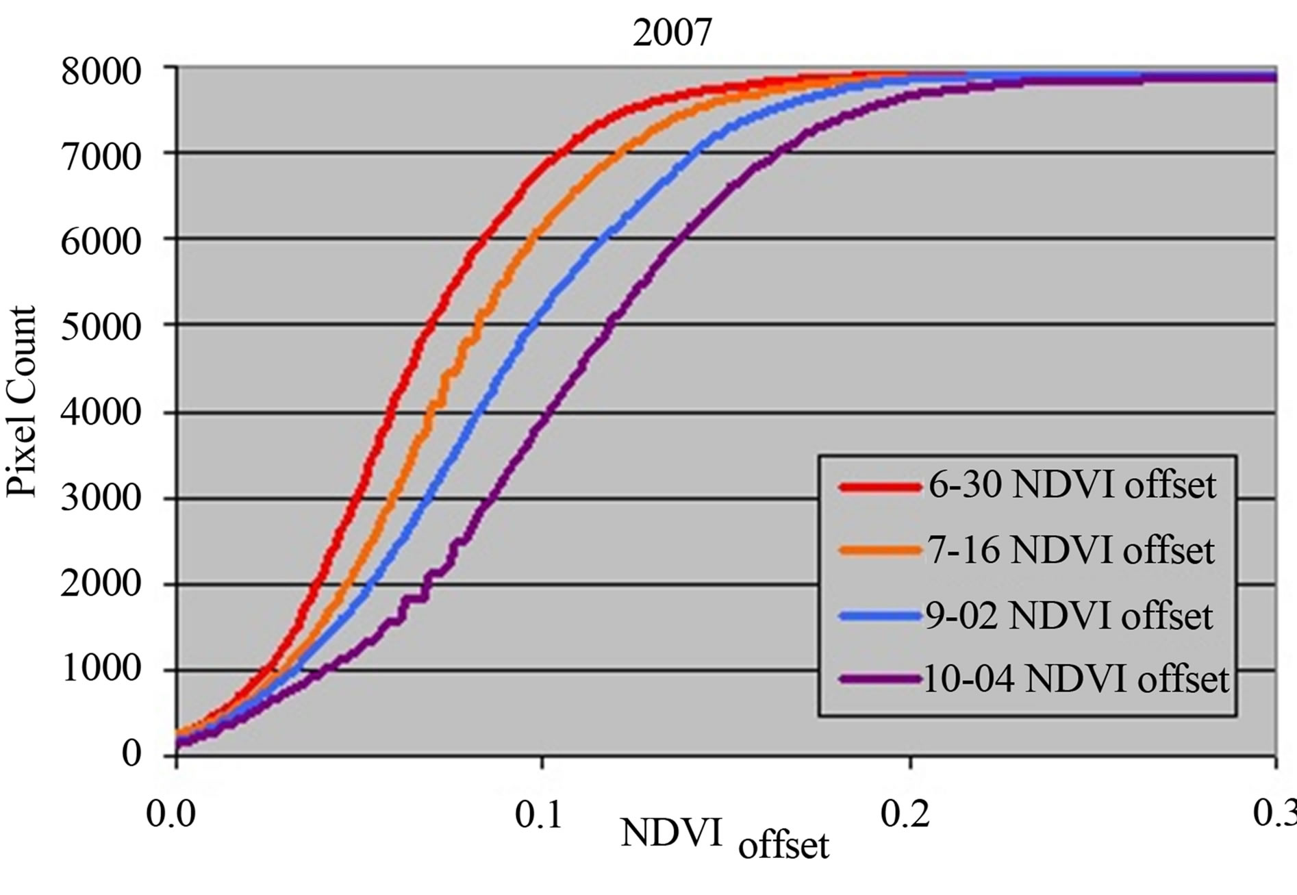
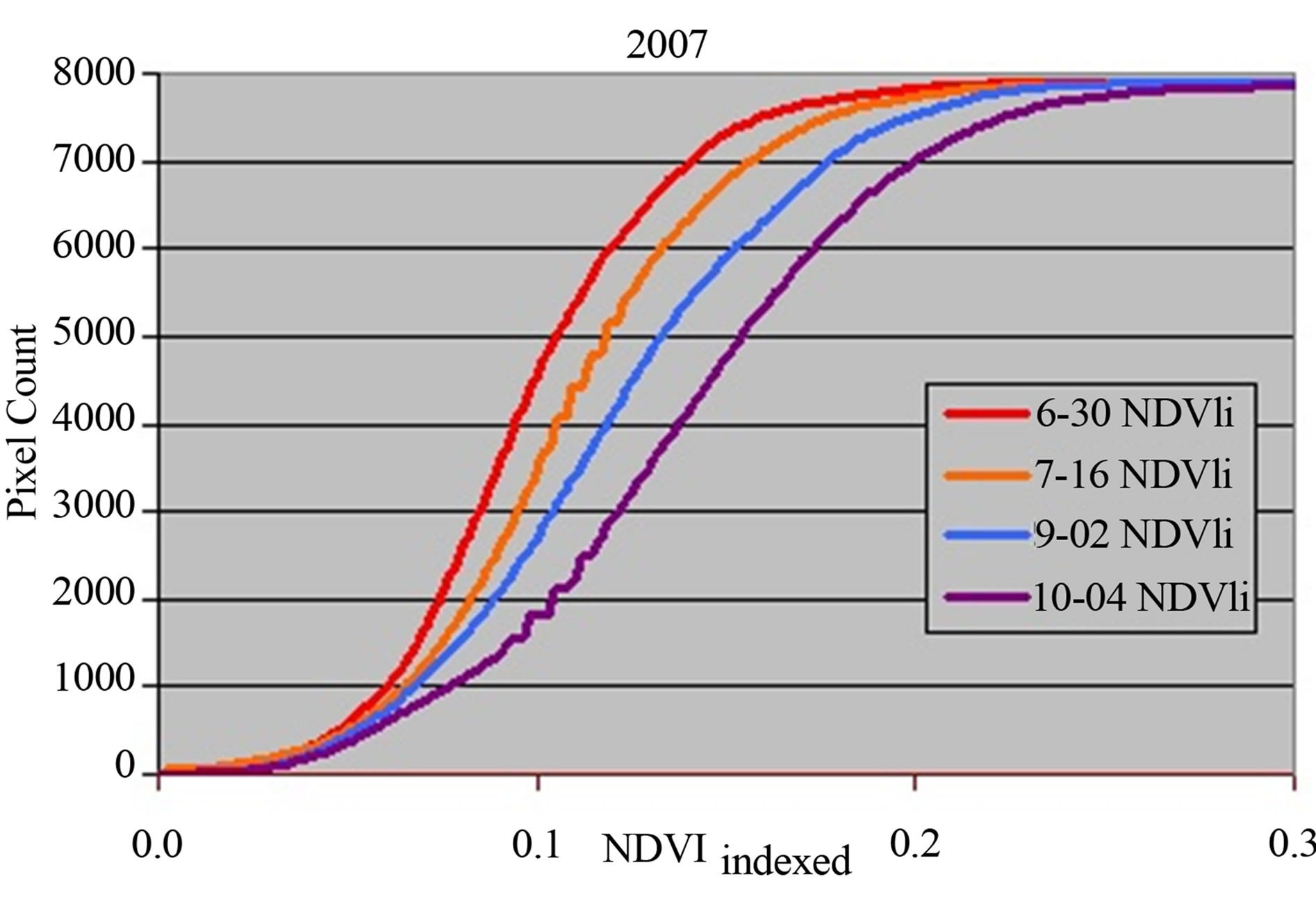
Figure 9. Three graphs of CDFs of NDVI that were generated for 2007, the benchmark year. Raw NDVI calculated from reflectance according to Equation 2 is shown in the top graph. Because of atmospheric effects and background soils, the curves do not increment in the expected order for MVA green cover that increased through summer to reach the annual peak in October. In the middle graph, NDVIoffset places the NDVI CDFs into the expected, incremental order peaking in October. Note that the NDVIoffset distribution is a first approximation that cuts the tails of these curves. In the lowermost graph, CDF curves are indexed to the 2007 NDVIoffset value and the 2007 estimated NDVI value for bare ground to yield NDVIx. The way to read these images is a rightward progression of the curves which denote increased green vegetation cover, while leftward progression denotes a decrease.
benchmark image was established by extraction of raw NDVI values from each of the late season images listed in Table 1. Two locations in the MVA, both devoid of vegetation, were chosen for this extraction. A ground view of a location used to measure the reflectance of a bare surface that was used is shown in Figure 10.
The value chosen for the standard, NDVIbare ground, was 0.0357, the NDVI value of bare soil measured on the benchmark 2007 EOS image (Table 2). This value was chosen because it was consistent with three other values that were extracted from the seven late season images; the average of the four being a very close value, 0.0355. Three divergent values in Table 2 were inconsistent and much lower than the four consistent values. These inconsistent values can be explained by NDVI depression from highly variable surface wetting, often occurring for these
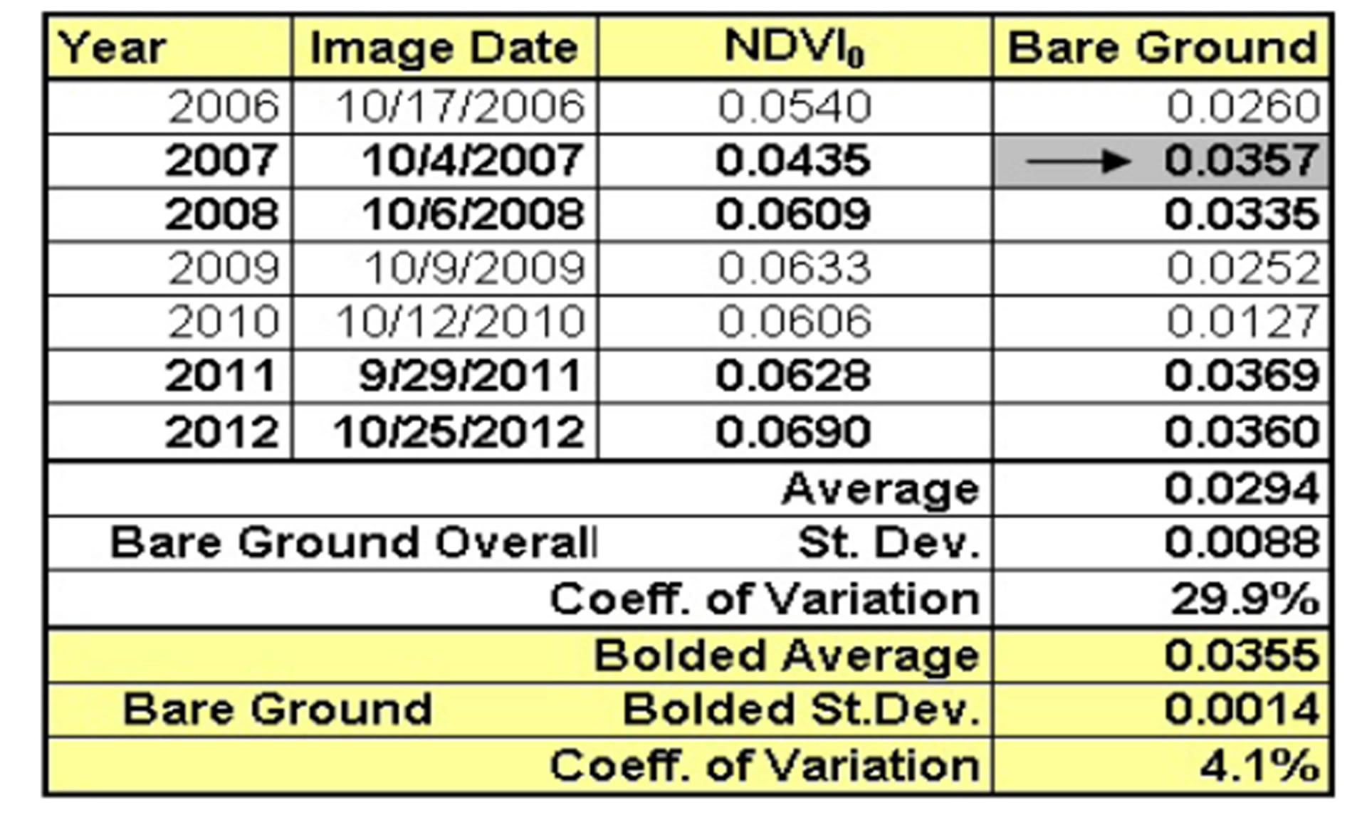
Table 2. NDVI bare ground NDVI extracted for each peak cover year. Bolded values have close numerical agreement. Statistics of bolded data are statistically tight while values that deviate from these four have lower magnitude and much greater variability. Coefficient of variation is group standard deviation divided by group average. Images were TM5 except for 2012 that was ETM7+.
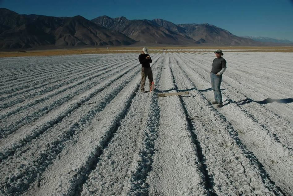
Figure 10. A January, 2007 view of a vegetation-free location used in calculation of NDVIx. The bare ground value was obtained two months prior to this photo. Salt enrichment of the surface was due to irrigation and poor drainage.
bare soil targets due to irrigation and poor drainage. Wetting on some of the divergent images in Table 2 was confirmed using Landsat Band 5, a surrogate measurement for surface wetting that is in use to judge compliance for shallow flood dust control of the Owens Lakebed [14].
Calculation of NDVIoffset for each pixel of each image collects the CDFs of all images together relationally as shown in Figure 9(middle). Calculation of NDVIx then indexes all values to the trusted bare soil value, 0.0357, measured on October 4, 2010 (Equation (3)) that corrects the CDFs of the images by re-shifting all images to the right by the same amount (Figure 9(bottom)). This removes truncation resulting from the NDVIoffset calculation. For the ith pixel and the jth image:
 (3)
(3)
The bracketed portion of Equation (3) is the formula for NDVIoffset. NDVIx that allows any image from any year to be compared to any other image.
2.5. Resampling to Grid Cells
After calculation of NDVIx for each image, the last procedure before making comparisons with the benchmark image was to resample the images to conform to the 0.405 ha grid cells. This operation was performed using the cubic convolution algorithm that was modified by an extra step in order to calculate a precise spatial average for the grid cell. Cubic convolution averages all centroid points that are included within a polygon, in this case a grid cell. Each acre contains 4.5 pixels whose centroids may be variously sampled through inclusion of 4, 6 or 9 pixels depending upon how rows and columns of pixel centroids fall into or are excluded from individual grid cells. This yields estimates of NDVIx that are systematically skewed inducing additional spatial uncertainty into the estimates, especially when comparing across years. This scaling-induced sampling problem was overcome by resampling each pixel into a 10 × 10 grid of 3-m pixels within each 30m Landsat pixel. This 100× finer grid was then resampled into 0.405 ha cells for a more precise and spatially-correct grid cell average.
3. Results
The data processing workflow for MVA vegetation performance has multiple steps and is relatively complex, so the first evaluation of the results was to confirm the validity of the estimates through the following steps:
1. Determine that the CDF curves incremented logically within each year, lacking any jumps from high to low to high or vice versa. Such jumps indicate unacceptable levels of uncertainty because vegetation in the target environment has not been observed to pulse in that manner.
2. Using the cover maps, compare to ensure that changes of vegetation cover within the system were logical. This is a spatial confirmation of the observations for the first step since patterns of high and low MVA vegetation growth have remained relatively unchanged in the period of operation.
3. On the cover maps, determine whether poorly performing areas, known to be constrained by poor drainage, shallow groundwater and salt buildup, have remained in the same location. Locations of poor vegetation growth are a more sensitive spatial indication of all factors that cause uncertainty, including geocorrection.
The first step was accomplished by examination of the CDFs for each year. The second step was evaluated as a combination of examining CDFs and examining maps of green vegetation cover. The third step was accomplished by examining acre grid cells for positions of low values, an exercise that is also useful to evaluate cover improvement or decline within problem areas.
3.1. CDF Curves and Logical Incrementation
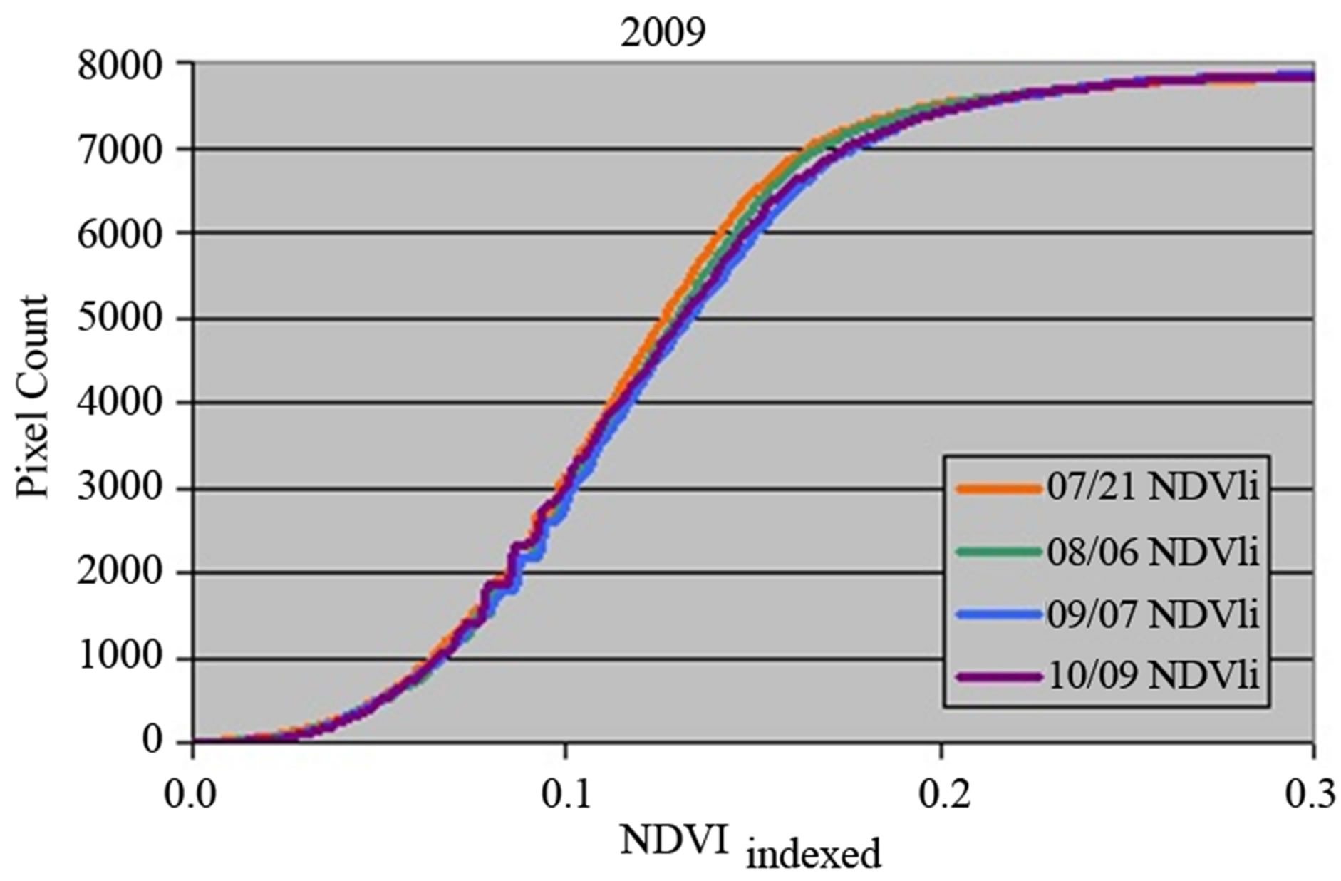
The annual CDFs for 2007 through 2012 showed that all monthly values incremented in a rational manner, with the lowest values of NDVIx occurring early in the season generally increasing to a peak in the summer or fall (Figure 11). No fluctuations occurred that could not be explained as the ebb and flow of normal growth.
Aspects of management, for example the timing of irrigation, can greatly influence the response of the vegetation. For example, during 2009, irrigation was reduced to test how water-thrifty MVA management could be. Reduction in water supply resulted in very little response for growing vegetation, indicating the direct relationship between MVA irrigation and canopy health. Different seasonal patterns for the CDF curves of Figure 11 are likely the responses to irrigation amounts, quality and timing.
The 2012 data shown in Figure 11 were generated with Landsat ETM7+ images that contained missing data stripes that were masked out of the calculations. The total pixel counts of the CDFs for 2012 lacked an average of 5.2% of the potential pixels within the MVA due to missing data stripes and so were scaled upwards to enable direct comparison with the Landsat TM5. The total correct number of pixels was about 7900. Pixel counts may vary according to the number of centroids of pixels included or excluded within the set 0.405 ha grid file of Figure 6.
3.2. Maps of Cover for 2007 through 2012
Figure 12 presents acre grid cell maps of the end-of-
 ;
; 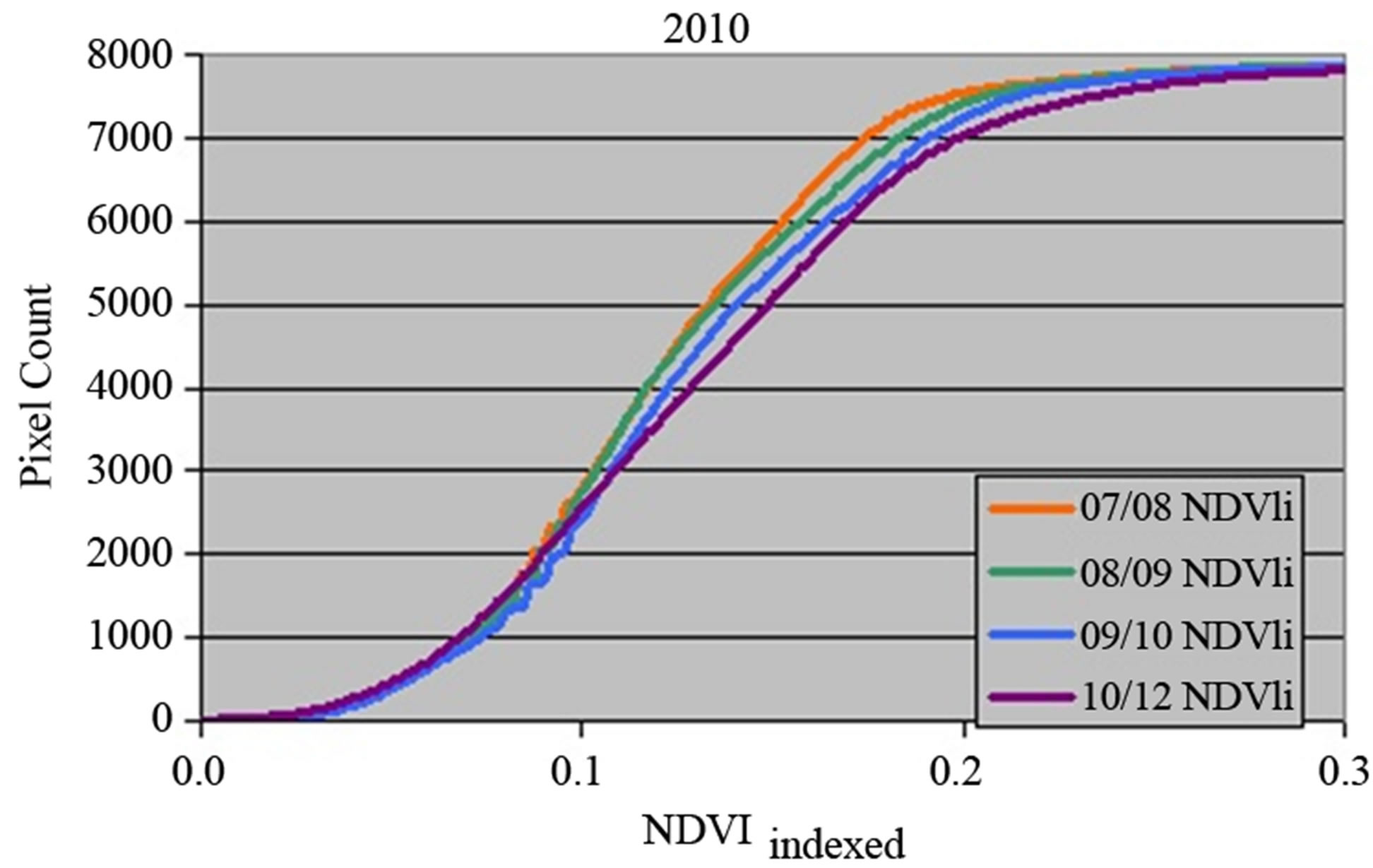
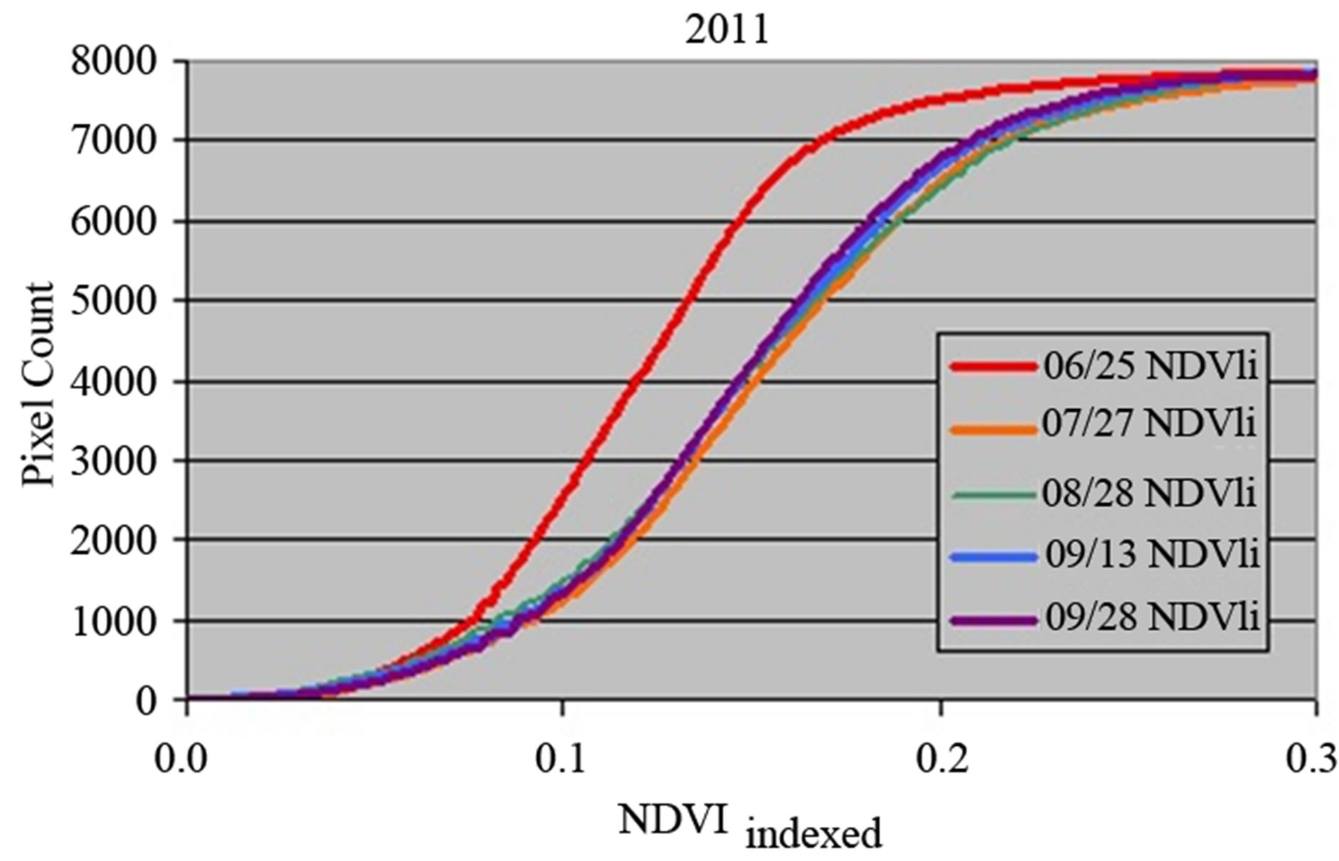
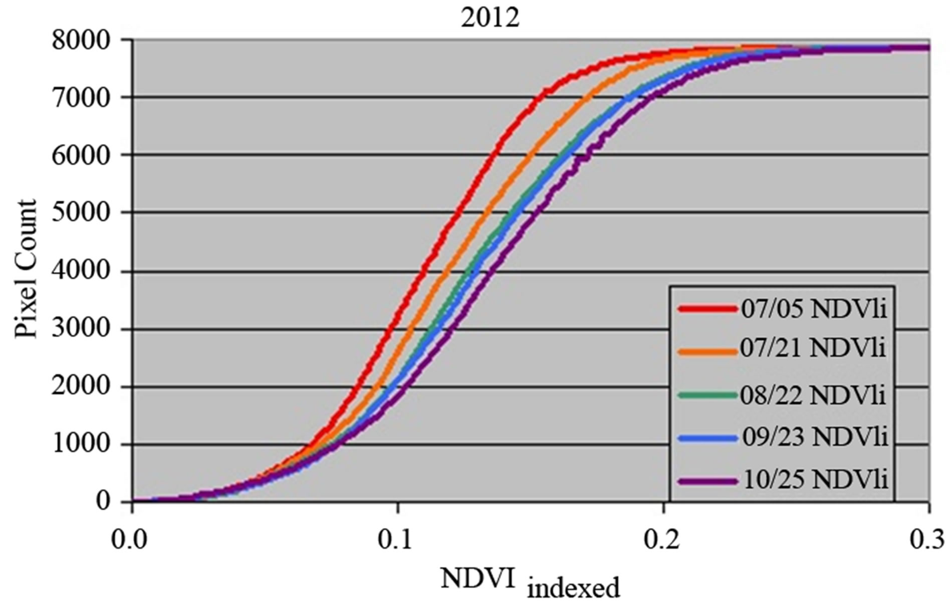
Figure 11. CDFs for 2007, the benchmark year and five years that follow. All images increment reasonably.
season vegetation cover across the MVA for the six years, 2007 through 2012. Examination of these images shows that the spatial vegetation performance follows the relative vegetation performance interpreted through examination of CDFs (Figures 9 through 12). Overall, the best performance occurred in 2011 and the poorest occurred in 2009.
Areas of very poor cover exist in the same locations year after year (Figure 12). These locations were identified as being caused by poor drainage leading to shallow groundwater that led to near surface salt buildup through capillarity. Given the acre grid cell discretization, these areas can be tracked by each individual acre to plan amelioration to foster more cover. However, since the “this or better” criterion is tied to 2007 and these areas lacked cover then, nothing different in management would be required.
The consistent spatial distribution of high and low vegetation performance confirms that the data are logical in a spatial sense, fulfilling the second step in the evaluation of the NDVIx processing.
3.3. Low Vegetation Cover, 2007 through 2012
The third step in the evaluation of the NDVIx processing methods was used to evaluate the distribution of the poorly performing vegetation cover. These are the areas with the highest potential to give rise to windborne dust within the MVA.
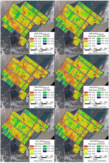
Figure 12. Mapped NDVIx on the MVA.
Patterns of low cover are due to drainage, shallow groundwater and salinity in static locations. Hence, examining patterns of low cover enables cross checking to determine the spatial accuracy of the NDVIx analysis. The maps displayed in Figure 13 show acre grid cells with cover less than 0.10 NDVIx displayed as transparent red. Locations with low 2007 vegetation cover are displayed as transparent blue and locations for 2007 and each comparison year are displayed as purple.
An examination of the areas in Figure 13 indicates
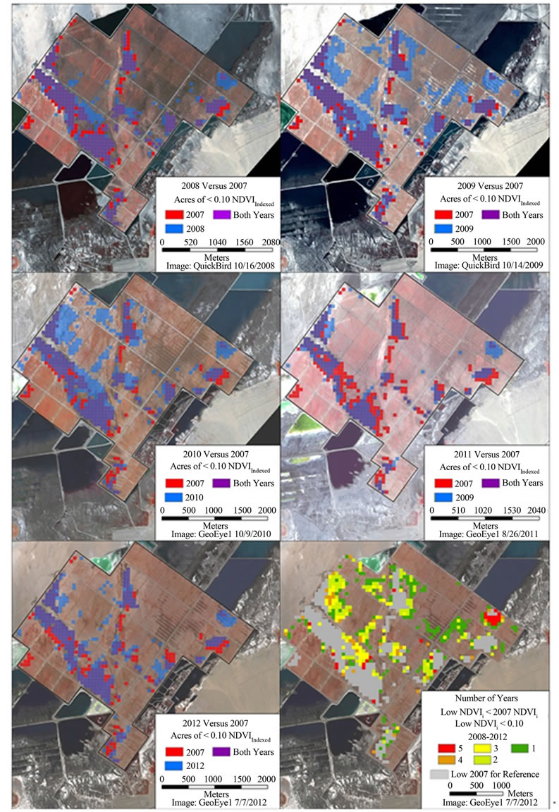
Figure 13. Locations of green growth less than NDVIx of 0.10 for each year, 2008 to 2012, compared to 2007. The map in the lower right corner is a composite of the five annual comparisons.
that areas of low cover have not changed significantly through the five-year period of this analysis, as expected. This provides spatial confirmation that processing the data to NDVIx provides accurate and dependable comparisons.
The acre grids of Figure 13 and especially the threshold level of 0.10 NDVIx, provide relatively coarse comparison relative to the CDFs of Figure 11 that enable much better discrimination at the important low end of NDVIx distribution. Red grid cells indicate improvement since 2007, while blue indicates poorer conditions. The spatial expression of improvement in the 2011 and 2012 maps shows that the improving (light gray) gridcells are found on the periphery of areas with low cover in 2007.
Both 2009 and 2010 contain much larger areas of acre grids that are expressed as blue, having less NDVIx response than in the 2007 benchmark year. The patterning of the blue colored acres, indicating decline from 2007 conditions, are in areas that were repeatedly below this benchmark year. Traces of these patterns are visible in all years.
The map at the lower right hand corner of Figure 13 is a composite image that shows the number of years that each acre experienced NDVIx less than 2007 benchmark conditions. There are two general foci of concern for management. An area of concern is located on the far east of the MVA experienced all five years with cover less than 2007. The complex light green to orange gridcells adjacent to the northwest border of the MVA and other areas surrounding the poorest growth zones should be watched for future changes.
3.4. Low Magnitude Vegetation Performance Judged by CDFs
CDFs, alone, provide a means to track relative performance of the MVA, and especially to detect whether vegetation has performed to par. Figure 14 presents the same CDFs as in Figure 11 with the lower end of the distribution scaled to facilitate interpretation. Again, it is the lower end of the distribution of the vegetation cover that is important for air quality.
From the CDFs of Figure 14 it is apparent that there is a great deal of variability among years. Also evident is that the 2007 peak expression of green cover has not always been attained in subsequent years. Of the five comparisons shown, only one exceeded 2007 growth (2011), two were equivalent to 2007 (2008 and 2012), and two failed to reach the 2007 green cover levels (2009 and 2010). Even though there is a range of growth that occurred each year, the lower portions of the six CDFs for 2007 through 2012 illustrate how tight the data are at the lowermost end of the distribution. All curves originnated from the same location near the origin and all incremented comparably to the peak-of-season growth in benchmark 2007 as is expected through the conversion of NDVIoffset to NDVIx.
The variability demonstrated in Figure 14 for attaining peak 2007 green cover levels illustrates that the three factors that can influence MVA saltgrass growth— amount, quality and timing of irrigation—need to be carefully managed in order to achieve growth at par with the 2007 benchmark. Otherwise, there is a 40% chance of failing to meet this goal (two in five years). The three irrigation-related factors mentioned above are the only factors that influence vegetation performance on the MVA since no pests or disease have been identified for the saltgrass, there is no grazing pressure, and the drainage and irrigation infrastructure have remained relatively unchanged through the five year period.
In Figure 14, it is apparent that the low MVA performance in 2010 may have been constrained by even lower performance in 2009. Canopy growth in 2010 may have still been impacted by the decreases that occurred the previous year, for example runners of saltgrass growth that failed and needed to regrow from a base that survived irrigation shortfalls. Another hypothesis is that the slow plant growth may have been due to irrigation practices that were extended into 2010. Combining irrigation records with these data offers the opportunity to identify MVA irrigation practices that should be avoided, and those that should be continued. The five years of vegetation growth offer the means to adjust irrigation quantity, quality and timing to achieve the green cover that existed in 2007 while conserving against an over supply that would waste water. Water conservation is an important goal in the Owens Lake second only to dust control.
Using the CDFs for evaluating compliance, reaching the 2007 par levels of green growth, is a simple and accurate way to evaluate the performance over the entire MVA. We know from Figures 12 and 13 that the patterns of high and low vegetation performance did not change markedly through the seven years and so, the CDFs can be expected to represent nearly the same grid cells, relationally, throughout the history of the MVA. In other words, at each given level of grid cell count, the CDFs compare about the same grid cells throughout the seven years. In these comparisons, 2012 appears to be optimal.
3.5. NDVIX Precision
CDF curves for 2009 were chosen as a means to evaluate the precision of the NDVIx processing. Because 2009 recorded very poor growth due to low water supply, the lowermost limb of the curves are measuring vegetation growth that essentially remains static through the grow-
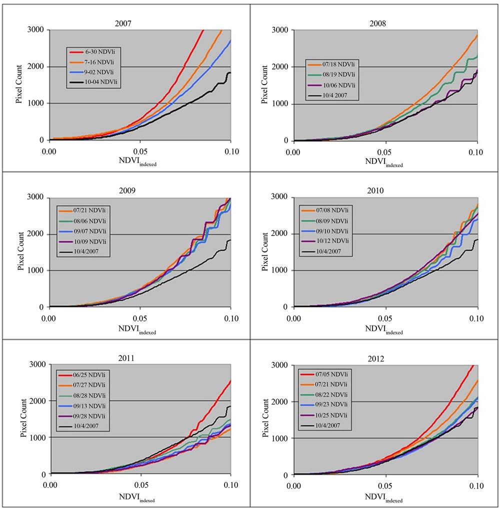
Figure 14. The lower portion of CDF curves for 2009, a year with stringent irrigation supply and quasi static growth response. Values for each curve were extracted in the locations indicated by the arrows.
ing season. Any apparent fluctuations in values can, therefore, be used to make a minimal estimate of precision—minimal, insofar as any differences may actually be the result of plant growth rather than statistical uncertainty. The graph shown in Figure 15 presents the same data for 2009 as shown in Figures 12 and 13 but with the lower limb enhanced to examine the variability of the curves. Four lines of equal pixel counts are indicated for 300, 400, 500, and 600 pixels in the region where the curves approach linearity. By assuming that these data represent no change in cover but simply the fluctuations resulting from uncertainty as the limit of precision for EOS data and NDVIx calculation is approached. An assessment of the variability at each of these four pixel count values provides an estimation of precision.
Table 3 calculates signal to noise ratio (SNR) for the data extracted at four pixel counts indicated in Figure 15. The measure of signal to noise is taken to be the mean as a representation of the signal, divided by the standard deviation, representing noise [15]. These data show that
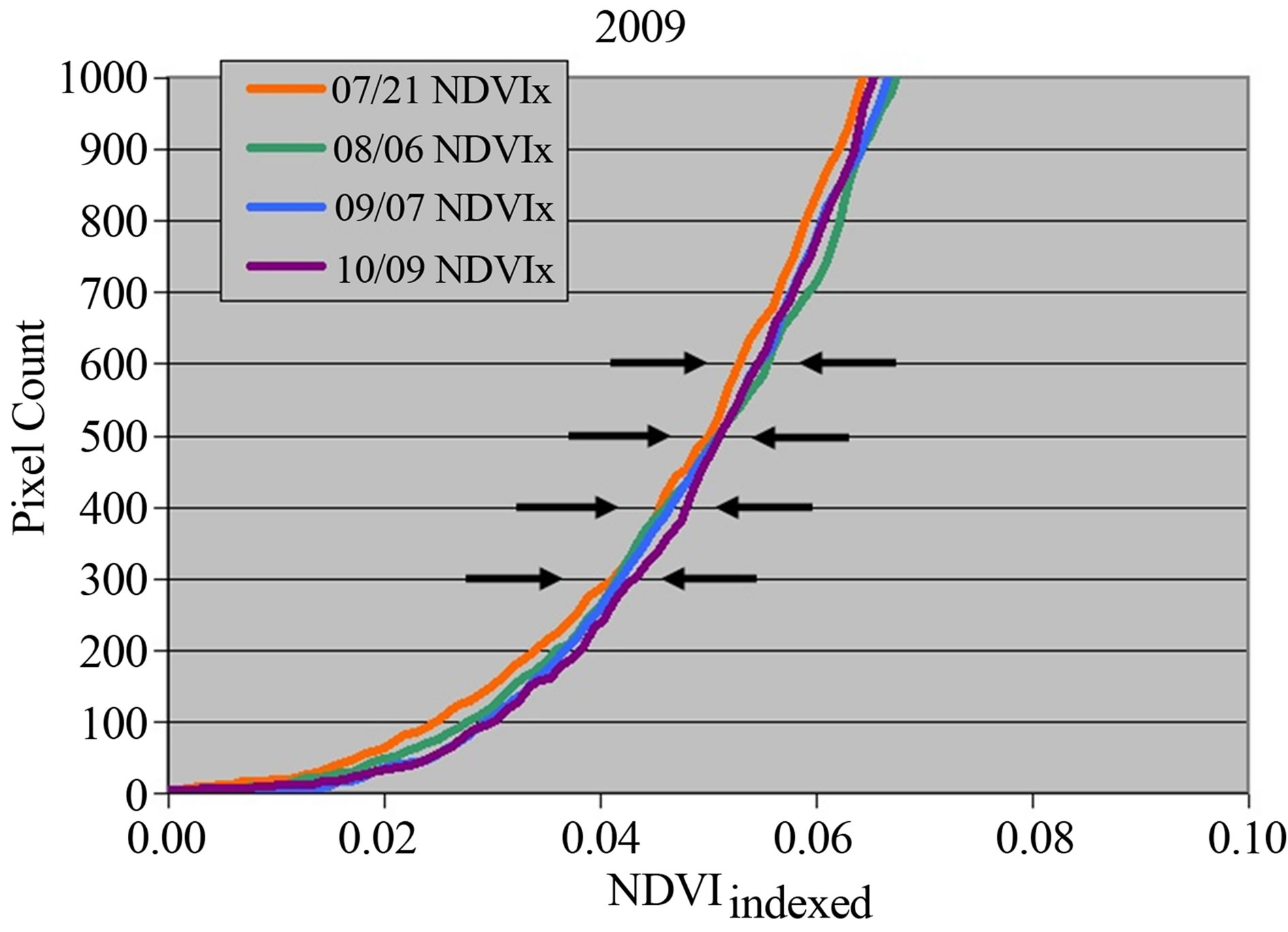
Figure 15. All CDFs displayed for the NDVIx region below 0.10. The black line in all graphs is the peak-of-season CDF from October 4, 2007.
the calculation of NDVIx has high precision with the average SNR of 64.2, but consistently at a level above 50. Again, since some of the differences in the CDF curves of 2009 (Figure 15) may be actual fluctuations, these values represent a minimal estimate of the SNR.
3.6. NDVIX, MVA Compliance, and Their Relationship to Air Quality
Deviating below the benchmark line of the 2007 peak season CDF has documentable consequences for air quality. Figure 16 presents an image that mates the 2010 dust camera results with low vegetation cover (0.075 NDVIx and below) detected in 2010. The dust camera program, operated by the District to identify blowing areas, has permanent digital video cameras mounted around the lake to identify blowing areas. The dust camera output transforms camera coordinate system into world coordinate system based upon a program developed by Corripio [16].
The threshold of 0.075 NDVIx was chosen through examination of the lower region of the CDFs shown in Figure 14 that experienced declines in NDVIx during 2010 from 2007 benchmark conditions. There is a moderately strong relationship between low vegetation vigor and the incidence of blowing dust. Although there are discrepancies in the locations shown by the dust camera mapping, it should be recognized that such dust source identification methods are only relatively accurate— actual field confirmation of evidence for dust release should also be gathered. The point made here is that documented areas of low cover have good potential to release fugitive dust.
The accuracy of the dust camera program suffers in some locations by lacking multiple views of the same dust source locations. For example, the red areas of high incidence for blowing dust in Figure 16 are closer to the
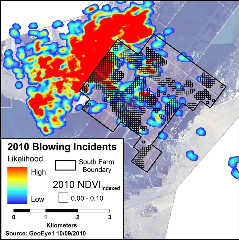
Figure 16. 2010 dust camera data for likelihood of dust release that are color coded for comparison to 0.405 ha grid cells identified to have low cover in 2010—north is to the top. Areas downwind (southeast) of highly active areas may be undercounted due to screening from blowing dust during windstorms.
camera position located to the northwest. Heavy releases of dust in the foreground of the dust camera images may, therefore, occlude active sources in the background during a windstorm.
There are mapped regions of dust release in 2010 that do not coincide with mapped areas of low vegetation in Figure 16. This may indicate that dust can be released from areas of thick vegetation cover. Such spot releases may result from wind vortices that entrain dust and salt crystals deposited on leaves of the vegetation. Salt crystal buildup on saltgrass leaves occurs naturally from excretion through glands on their upper surfaces. Hence, although vegetation is effective in reducing fugitive dust, it may contribute dust during high winds depending on the degree of buildup of dust and salt crystals in the canopy. Such mapped areas may generally have low likelihood for emitting dust but may do so under special circumstances.
Dust emission from the MVA may contain a large component of re-entrained particles. This is borne out by the worst areas for dust release being the locations along the northwest edge of the MVA that received significant particle deposition from northerly winds during 2010. Figure 16 shows areas of high activity dust release as red. The largest of these areas arose from wind entrainment to the northwest of the MVA that translocated up to a meter depth of soil onto the MVA where it partially buried vegetation and continued to be an active dust source during the 2010-2011 dust season.
3.7. Proposed Monitoring Program for Vegetation Compliance
At the time of this paper, the monitoring program is undergoing review for a potential upgrade to accommodate the results from this research. A logical step for monitoring using NDVIx would have the following steps:
1. Processing as described in this paper to arrive at NDVIx within the set acre grid cells and after removal of pixels potentially influenced by edge affects.
2. Comparison by subtraction from the October 10, 2007 acre-wise NDVIx to determine whether each acre grid cell has increased or decreased.
3. Extraction of acre grid NDVIx and display as CDF for comparison to 2007 conditions.
4. Display NDVIx for the year in question and NDVIx for 2007 (as in Figure 11). A curve to the left of the 2007 curve falls short of par.
5. Display the NDVIx difference map (as in Figure 12) to check for changes that may form patterns of concern.
6. Repeat steps 4 and 5 for NDVIx of less than 0.1 (as in Figures 13 and 14). Such locations of low cover are more critical for air quality.
4. Conclusions
NDVIx is proposed as the standard for assessing vegetation on the MVA because it is a highly accurate metric of vegetation performance that was shown to be superior to other methods tested in this work and in other comparisons. Because NDVIx is an index of green vegetation cover, it must be applied during the growing season. To identify and measure peak green vegetation cover, multiple images obtained during the growing season can be evaluated in order to catch the true peak, especially if this occurs at a different time than have typically occurred at the MVA—at season end. Because satellite data are archived, this reconstruction can take place after the growing season has ended. Verification that CDF curves increment logically provides a quality assurance step for the data processing.
Assessment of MVA vegetation performance using NDVIx requires the following steps for each image to be compared:
1. Select and acquire appropriate EOS imagery.
2. Geocorrect imagery by image to image registration with a standard base image.
3. Display the image in 432 RGB to examine for haze or other visible aerosols.
4. Convert the image to reflectance.
5. Calculate NDVI.
6. Display NDVI as a CDF.
7. Calculate NDVI0 for the image using a set regression interval.
8. Subtract NDVI0 from all NDVI values to yield NDVIoffset.
9. Add 0.0357, the benchmark image’s bare soil value, to index the images.
10. Screen out pixels that may contain non-vegetated surfaces of roadways and areas outside of the MVA boundary.
11. Resample each pixel using cubic convolution to a higher resolutions—a 10 × 10 resampling was performed for this paper.
12. Resample the 100x pixels into 0.45 ha grid cells using cubic convolution.
The results from these measurements indicated poor vegetation response in 2009 that carried over into 2010. MVA performance in both years failed to equal or better the benchmark year of 2007. Carryover of lower cover vegetation into 2010 may have played a role in 2010 dust releases documented to have been generated in the MVA. Comparison of irrigation records from good and poor vegetation growth years should be performed to assure that the vegetation cover in all future years remains at or above the 2007 levels.
5. Acknowledgements
The authors thank the Great Basin Unified Air Pollution Control District and staff for supporting this work, especially Ted Schade, Air Pollution Control Officer and Grace McCarley-Holder, Geologist.
REFERENCES
- C. A. Pope, D. W. Dockery, J. D. Spengler and M. E. Raizenne, “Respiratory Health and PM10 Pollution: A Daily Time Series Analysis,” The American Review of Respiratory Disease, Vol. 144, No. 3, 1987, pp. 668-674.
- W. L. Kahrl, “Water and Power,” University of California Press, Berkeley, 1982.
- H. S. Gale, “Salines in the Owens, Searles and Panamint Basins, Southeastern California,” US Geological Survey Bulletin 580, 1915, pp. 251-323.
- A. S. Jayko and S. N. Bacon, “Late Quaternary MIS 6-8 Shoreline Features of Pluvial Owens Lake, Owens Valley, Eastern California,” In: M. C. Reheis, R. Hershler and D. M. Miller, Eds., Late Cenozoic Drainage History of the Southwestern Great Basin and Lower Colorado River Region: Geologic and Biotic Perspectives, GSA Special Papers 439, 2008, pp. 185-206. http://dx.doi.org/10.1130/2008.2439(08)
- P. Saint-Amand, C. Gaines and D. Saint-Amand, “Owens Lake, an Ionic Soap Opera Staged on a Natric Playa. Centennial Field Guide,” Cordilleran Section of the Geol. Soc.Am., Vol. 1, 1987, pp. 145-150.
- Great Basin Unitified Air Pollution Control District, “2003 Owens Valley PM10 Planning Area Demonstration of Attainment State Implementation Plan,” 2013. http://www.gbuapcd.org/Air%20Quality%20Plans/2008SIPfinal/2008%20SIP%20-%20FINAL.pdf
- Soil and Water West Incorporated, “Owens Lake Bed Soil Survey,” 2013. ftp://gbuapcd.org/HydroReports/Soil%20Survey%202000.pdf
- California Irrigation Management Information System, “Monitoring Data from Owens Lake,” 2013. http://wwwcimis.water.ca.gov/cimis/welcome.jsp
- D. W. Goodall, “Some Considerations in the Use of Point Quadrats for the Analysis of Vegetation,” Australian Journal of Biological Sciences, Vol. 5, No. 1, 1952, pp. 1-41.
- W. M. Baugh and D. P. Groeneveld, “Broadband Vegetation Index Performance Evaluated for a Low-Cover Environment,” International Journal of Remote Sensing, Vol. 27, No. 21, 2006, pp. 4715-4730. http://dx.doi.org/10.1080/01431160600758543
- D. P. Groeneveld and W. M. Baugh, “Correcting Satellite Data to Detect Vegetation Signal for Eco-Hydrologic Analyses,” Journal of Hydrology, Vol. 344, No. 1, 2007, pp. 135-145. http://dx.doi.org/10.1016/j.jhydrol.2007.07.001
- D. P. Groeneveld, “Remotely-Sensed Groundwater Evapotranspiration from Alkali Scrub Affected by Declining Water Tables,” Journal of Hydrology, Vol. 358, No. 2-3, 2008, pp. 294-303. http://dx.doi.org/10.1016/j.jhydrol.2008.06.011
- R. Irish, “Landsat 7 Science Data Users Handbook,” 2013. http://landsathandbook.gsfc.nasa.gov/data_prod/prog_sect11_3.html
- D. P. Groeneveld, R. P. Watson, D. D. Barz, J. B. Silverman and W. M. Baugh, “Assessment of Two Methods to Monitor Wetness to Control Dust Emissions, Owens Lake, California,” International Journal of Remote Sensing, Vol. 31, No. 11, 2010, pp. 3019-3035. http://dx.doi.org/10.1080/01431160903140787
- D. C. Montgomery, “Design and Analysis of Experiments,” 4th Edition, Wiley, New York, 1997.
- J. P. Corripio, “Snow Surface Albedo Estimation Using Terrestrial Photography,” International Journal of Remote Sensing, Vol. 25, No. 24, 2004, pp. 5705-5729. http://dx.doi.org/10.1080/01431160410001709002