Journal of Mathematical Finance
Vol.3 No.2(2013), Article ID:31842,6 pages DOI:10.4236/jmf.2013.32032
How Intangible Dynamics Influence Firm Value
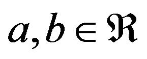
Department of Accounting, Feng Chia University, Taiwan
Email: nsshih@fcu.edu.tw
Copyright © 2013 Nien-Su Shih. This is an open access article distributed under the Creative Commons Attribution License, which permits unrestricted use, distribution, and reproduction in any medium, provided the original work is properly cited.
Received March 7, 2013; revised April 16, 2013; accepted April 29, 2013
Keywords: Value Relevance; Intangible Assets; Optimal Control
ABSTRACT
This paper analyzes the effect of changes in intangible assets on the relationship between the market value of a firm and its book value from a conservative accounting perspective. We find the value of intangible assets to have a positive association with the book value of operating assets and cash dividends. Firms with higher values related to intangible assets generally have more book value related to operation assets and cash dividends. Our evidence indicates that intangible assets are value relevant, i.e., they are associated with the market value of a firm.
1. Introduction
Previous research on the value relevance of intangible assets has provided evidence that omission of intangibles from a balance sheet is a serious deficiency, particularly because value for modern businesses is seen to come more from an intangible asset base than from physical assets (e.g., Abody and Lev [1]; Wyatt [2]; Penman [3]). Proponents of the capitalization of intangibles argue that earnings that reflect the effects of this capitalization are significantly more highly associated with stock prices and returns. On the other hand, a high level of uncertainty associated with future benefits might lead to managerial errors with regard to the amount of capitalization, and intangibles are difficult to verify independently of the value of firms (Jone [4]; Ciftci [5]). There is therefore potentially a significantly higher incidence of earnings management and financial misstatement. Hence, the impact of the capitalization of intangibles on the valuation of firms and quality of accounting is unclear. Our objective in this study is to provide direct evidence intended to aid in resolving this problem by analyzing how the value of intangibles affects the relationship between the market value of a firm and its book value.
Feltham and Ohlson [6] used a given relation between operating and financial assets for evaluating firm value (hereafter the FO model) in which the relative weights between a firm’s operating and financial assets on equity will affect future distributions of earnings, and thus affect the valuation of a firm. A change in intangible assets not only affects the relative weights between operating and financial assets, but also affects the quality of accounting information and the value of a firm. However, this given relation is time dependent and will change as time passes. Empirical evidence has also indicated that the valuation function is not linear (e.g. Burgstahler and Dichev [7]; Collins et al. [8]). Therefore, we develop a dynamic model on optimizing behavior to overcome the limitations of the FO model by emphasizing the role of intangible assets. Our model explains how a firm’s ownermanager incorporates intangible assets into the valuation of a firm, and aids in determining whether the optimal relation between operating assets and financial assets is affected by intangible assets. The results of our analyses reveal that, under long-term stable equilibrium, the operating and financial activities of the firm will adjust in relation to optimization, and the marginal utility of cash dividends as well as operating and financial assets will gradually be congruent. Consistent with theory, we find that intangible assets influence the weight of operating assets on book value of equity. The more intangible assets a firm has, the more operating assets it will have, and the higher value of the firm will be.
This study contributes to the literature in two regards. First, by developing a formal valuation model to overcome the limitations of prior literature, we are able to examine the valuation function and its cross-sectional dynamics more broadly, and to propose the theoretical support for the empirical findings in related studies. Second, focusing on exploring the impact of intangible assets on market value of firms and quality of accounting information, this paper can provide theoretical support to accounting reform in regard to value relevance for standard setters.
The rest of the paper proceeds as follows: In Section 2, we lay out the basic assumptions and settings of our model. Section 3 describes the dynamic process of our model. In Section 4, we analyze the impact of intangible assets. Concluding comments are stated in Section 5.
2. Theoretical Model
In this section, we set up an intertemporal dividends valuation model for a firm subject to constraints of operating assets, financial assets and intangible assets. We solve the optimal control problems of this model to determine the firm value.
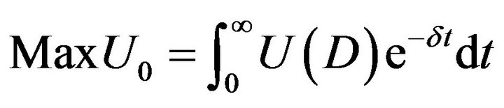
Stock price is determined as the present value of a stream of future cash flows. A firm provides its shareholders future cash flows made of a stream of dividends until the firm is liquidated or sold. Therefore, the value of a stock can be determined as the present value of an infinite stream of dividends. Follow Abel [9], Abel and Blanchard [10], and Sen and Turnovsky [11], we assume that a principle, who is the firm’s owner and also a manager, has the ability of forecasting his/her firm’s future cash flows. Under the going-concern assumption, the owner-manager of the firm will receive cash dividends and cause an increase in utility in each period. Therefore, the problem is to choose a sequence of dividends that will maximize the present value of the utility. The owner-manager’s decision can be determined by solving the following intertemporal optimization problem:
 (1)
(1)
where  is time preference rate of the owner-manager of the firm, assumed to be constant.
  is the utility function of cash dividend D for the owner-manager of the firm.
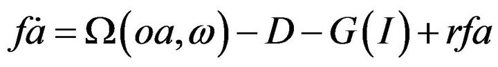
Feltham and Ohlson (1995) built a model that connects a firm’s market value and the accounting data related to operational and financial activities. A firm’s book value of equity is considered to be equal to the sum of book value of operating assets (oa) and financial assets (fa)1. In the FO model, financial assets can only have normal returns. Abnormal earnings are generated only from the operating assets of a firm. Since conservative accounting induces bias, it will reduce the book value of operating assets. Under unbiased accounting, the book value of a firm is equal to its market value. Conservative accounting systematically understates the value of operating assets so that book value of the firm is lower than its market value. Consistent with Feltham and Ohlson (1995), we assume that the accounting measurements satisfy the clean surplus relation. The change of operating assets  is equal to earnings from operating activity (Ω) less cash flows transferred to the financial assets (C). i.e.,
  , where
  is the exogenous variable representing the market value of intangible assets and where
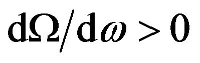 , indicating that increases in the market value of intangible assets will cause an increase in operating income.
 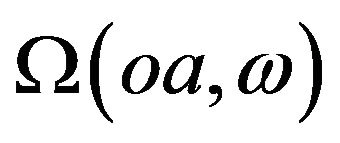 represents the firm’s operating income, which is assumed to be a continuation function so that
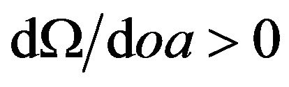 , reflecting that increases in operating assets will make operating income increase, and
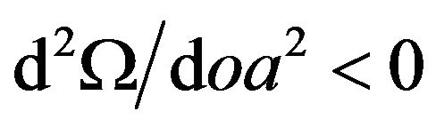 , reflecting that the speed of operating income increase will be slowed down as operating assets increase. Since the cumulative process of operating assets requires some costs (C) for adjustment2, the change of operating assets
  can be expressed as:
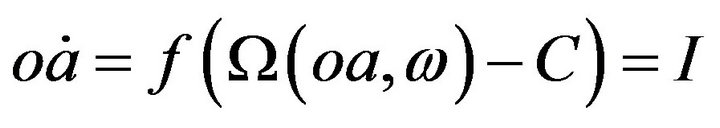 (2)
(2)
Assuming G function is an inverse function of , Equation (2) can be rewritten as:
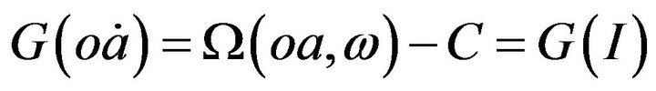 (3)
(3)
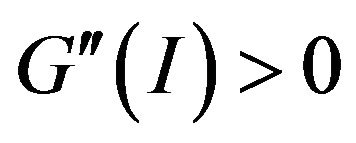
The function 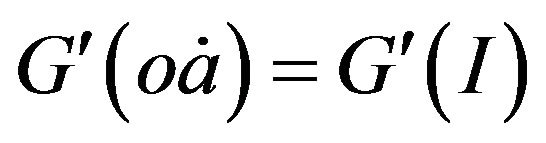 represents the additional installation costs associated with I units of purchase for new operating assets. Assume G(I) is an increasing and convex function such that
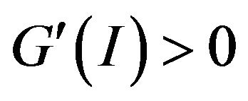 ,
, . In addition, we assume that at the initial point,
 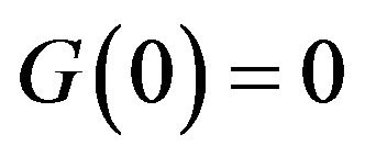 , and
, and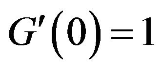 . i.e.; the total cost of no investment in operating assets is zero, and the marginal cost of the initial installation is unity3.
According to the assumptions of financial assets relation (FAR, see Feltham and Ohlson, 1995), financial activities can only have normal returns and thus the book value of financial assets will equal to its market value. FAR states that (operating) cash flows increase financial assets, whereas dividends reduce financial assets4. Therefore, the change in financial assets  can be written as
 (4)
(4)
Without considering the measurement bias under conservative accounting, the market value of the firm will be equal to its book value (bv), which is the sum of the operating and financial assets. According to the FO valuation model, the value of intangible assets, i.e. goodwill, depends on the accounting principles employed. Under conservative accounting, the market value of a firm is equal to its book value plus the value of intangible assets. Therefore, the value of intangible assets  will be equal to the difference between the market value of the firm and its book value. Assume that the beginning financial assets is
 , and the beginning operating assets is
 . The problem of the firm’s ownermanager is to choose a sequence of dividends that maximizes the present value of utility by using the maximum principle of Pontryagin. That is,
Subject to
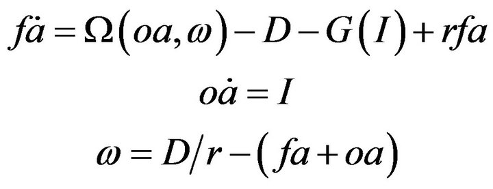 (5)
(5)
The Hamiltonian function (Kamien and Schwartz, 1991) for this problem is:
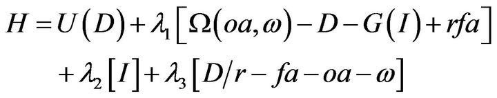 (6)
(6)
where ,
,  and
and , the costate variables associated with Equation (5), are the shadow prices of financial assets, operating assets and intangible assets, respectively.
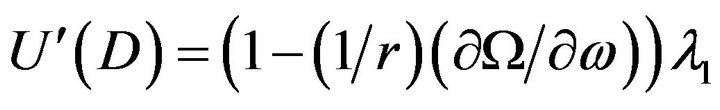
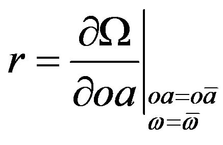
That is, as one-unit increases in financial assets, operating assets, or intangible assets, the units increase in regard to the utility of the owner-manager of the firm. The first step in the solution process is to take the partial derivatives of the Hamiltonian function with respect to each dividend (D), investment (I) and the intangible asset  variables and set each of these partial derivatives as equal to zero. The optimal conditions of this model can be rewritten as follows:
 (7)
(7)
 (8)
(8)
Equations (7) and (8) define the short-term equilibrium of the system. Equation (7) equates the marginal rate of substitution of dividends to the shadow price of financial activities, and Equation (8) equates the marginal cost of operating activities to the marginal price of operating activities. From Equation (8), we can infer that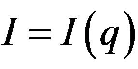 and
and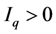 . That is, because the marginal utility of operating activities is higher than that of financial activities, the firm will put more capital into the operating assets.
3. Equilibrium Dynamics
Carrying out the procedure outlined above, this framework can be used for locating the dynamic path of q, oa and fa. Letting  be the equilibrium points of
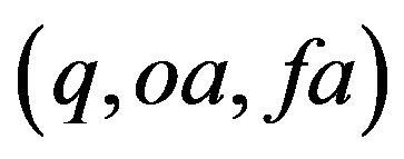 , the linearized differential equations around the steady state are written as Equation (9), where all derivatives in the matrix are evaluated at the steady state, and where
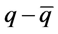 ,
,  , and
, and  are deviations of q, oa, and fa from their respective steady state values. We can therefore obtain:
 (10)
(10)
The dynamic characteristics of the system depend on the sign of (q – 1). There are three cases concerning the sign of (q – 1): (q – 1) > 0, (q – 1) = 0 and (q – 1) < 0, which are discussed as follows:
CASE 1: (q – 1) = 0
If (q – 1) = 0, three roots (v1, v2 and v3) may be (1) three negative roots (Case 1.1), or (2) two negative roots and one positive root (Case 1.2), or (3) two complex roots and one positive root (Case 1.3).
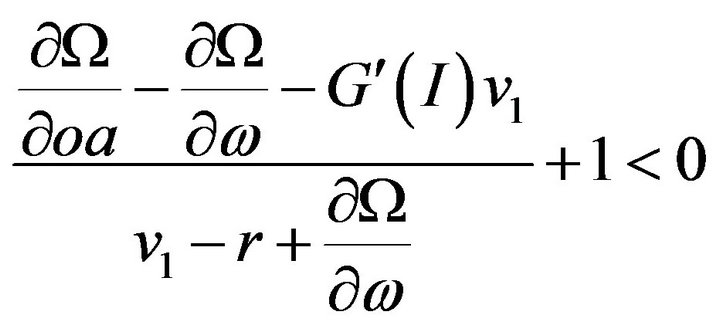
Case 1.1 A situation of (three positive roots) is impossible since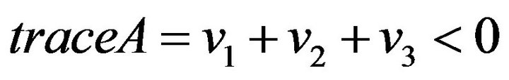 , and this equation would therefore be violated.
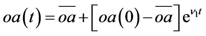
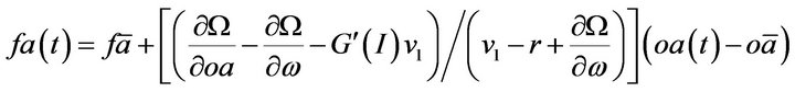
Case 1.2 (two negative roots and one positive root) infers that  is a saddle point equilibrium with a unique path to the steady state. Letting v1, v2 and v3 be roots of this equation, and v1, v2 < 0 < v3,
 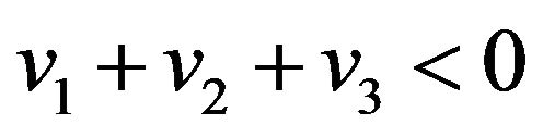 , we can show that the optimal path to a steady state is as follows:
 (11)
(11)
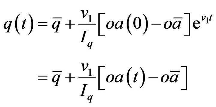 (12)
(12)
|
|

 (13)
(13)
and the time trajectory for ,
,  and
and  are shown in Figure 1. There exists a negative relationship between
  and
and  since
since ,
, . That is, as
  increases,
  will decrease. As
  increases,
  will decrease. There is an opposite relationship between
  and
and , in which an increase in operating assets reduces the demand for financial assets. This means that a firm’s operating assets and financial assets are mutually substitutive. When a firm invests more on financial assets, it must cut investment in operating assets, and vice versa.
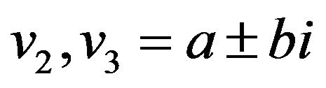
Case 1.3 (two complex roots and one positive root) Letting v3 > 0, 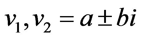 ,
,  , and 2a + v3 < 0, we can infer that
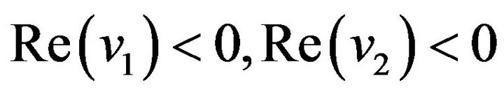 , and that
  is a saddle equilibrium point. From Case 1.3, we get the solutions in Case 1.3 for
 ,
,  and
and , which are similar to Case 1.2.
CASE 2: (q – 1) < 0
If (q – 1) < 0, we have the same results as Case 1.
CASE 3: (q – 1) > 0
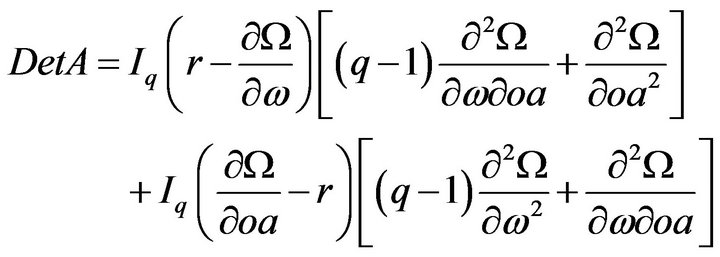
Since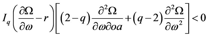 there are two possibilities for Det A. If Det A > 0, we can get the same results as Case 1. If Det A < 0, we have three roots that may be (1) three negative roots (Case 3.1), or (2) two positive roots and one negative root (Case 3.2), or (3) one negative root and two complex roots (Case 3.3).
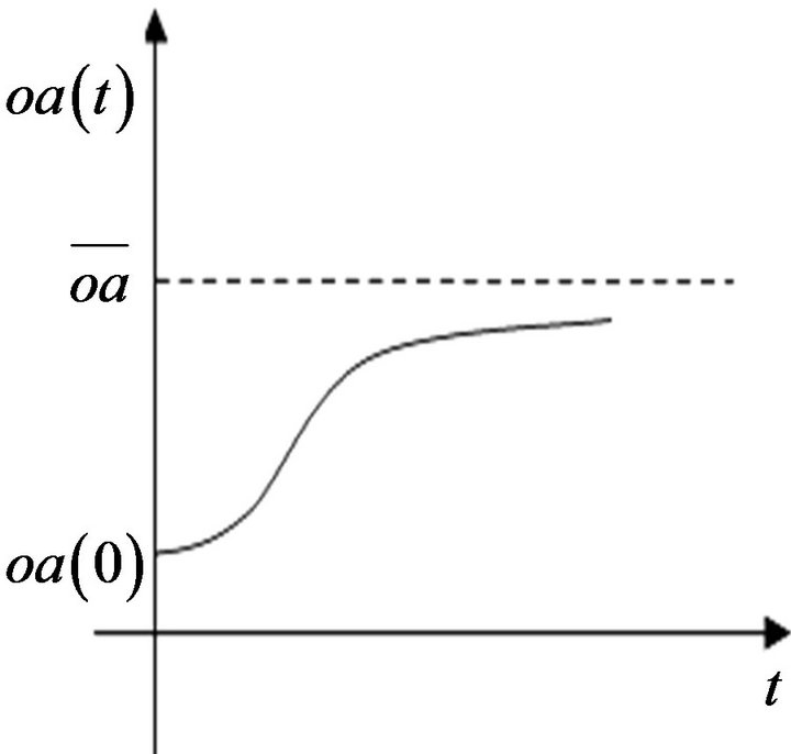
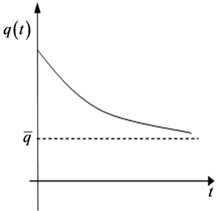
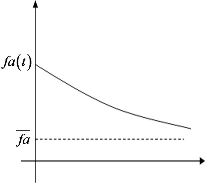
Figure 1. The time trajectory of , the time trajectory of
  and the time trajectory of
 .
.
Case 3.1 (three negative roots) infers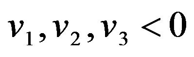 . This implies
  is an attractor equilibrium point. Similar to Case 1.2, we can get the phase diagram for oa(t), q(t) and fa(t), as shown in Figure 2.
Case 3.2 (two positive roots, one negative root) infers that 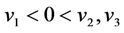 and
and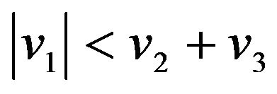 . Solutions for Case 3.2 are similar to those of Case 1.2, and
  is a saddle equilibrium point. The phase diagrams for oa(t), q(t) and fa(t) are displayed in Figure 3.
Case 3.3 (one negative root, two complex roots) infers that ,
,  and that
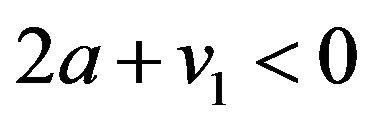 . This implies that
  is a saddle equilibrium point whenever a > 0, or that
  is a attractor equilibrium point whenever a < 0. Similar to Case 1.2, Figures 4 and 5 show the phase diagrams for
 ,
,  and
and  in Case 3.3.
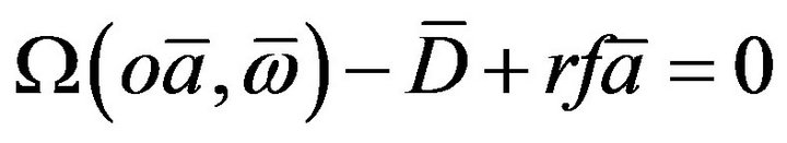
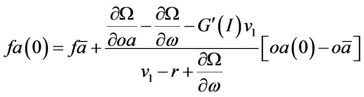
4. The Impact of Change on Intangible Assets
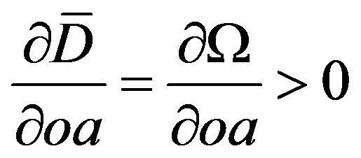
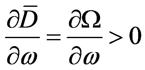
This section focuses on analyzing the impact of change in intangible assets on operating assets and the steadystate equilibrium of the system. From the foregoing necessary condition (5), we can get
 (14)
(14)
The relationship between  and
and  can be observed in Figure 6. It is a positive relation. That is, as operating assets
  increase, intangible assets
  will increase as well. The condition for equilibrium in the system is that
 . Then the necessary conditions to satisfy the optimality are:
 (15)
(15)
 (16)
(16)
 (17)
(17)
 (18)
(18)
 (19)
(19)
This yields the following implement ability condition:
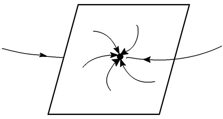
Figure 2. The phase diagram for ,
,  and
and  in Case 3.1.
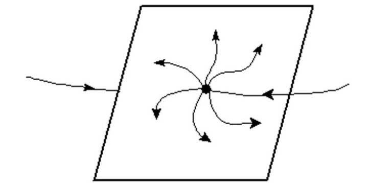
Figure 3. The phase diagram for ,
,  and
and  in Case 3.2.
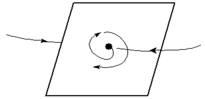
Figure 4. The phase diagram for ,
,  and
and  whenever a > 0.
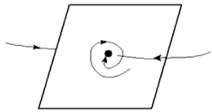
Figure 5. The phase diagram for ,
,  and
and  whenever a < 0.
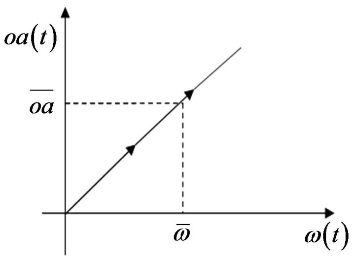
Figure 6. The relationship between operating assets and intangible assets.
 ,
,  , and
, and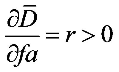 .
.
This means that as the value of a firm’s intangible assets  increase, its operating assets
  will increase too. In addition, the firm’s dividend distribution (D) is positively associated with its intangible assets and operating assets. Increase in intangible assets and operating assets will raise the profit of a firm, so that dividends are also increased and vice versa. This result implies that the higher the intangible assets of the firm are, the higher the firm’s market value will be. The book value of intangible assets understates its market value due to accounting conservatism. This gap between book value and market value of intangible assets will deteriorate the quality of accounting information.
5. Conclusion
This study develops an optimizing model to analyze the effect of change on intangible assets in the intertemporal optimizing relation between operating assets and financial assets, and the effect of change on intangible assets on firm value. Our results show that, in the case of shortterm equilibrium, if the marginal utility of operating activities of a firm is larger than that of financial activities, then the firm will retain earnings instead of distributing cash dividends and will also invest more capital in operating assets. In long-term equilibrium, a firm’s operating and financial activities are adjusted to optimal scales, and the marginal earnings will be equal to the rate of time return at long-term equilibrium. Our results suggest that the relation between intangible assets and operating assets is positive. As a firm’s intangible assets increase, the relative return rate for operating assets to that for financial assets will also be enhanced. Therefore, a firm will increase its investment in operating assets. In addition, as a firm’s intangible assets and operating assets increase, it will distribute cash dividends in the future and thus raise firm value. This implies that the more intangible assets a firm has, the higher the firm value will be. However, the book value of intangible asset understates its real value due to accounting conservatism and thus deteriorates the value-relevance of accounting information. This result provides analytical support for prior empirical research (e.g. Collins, et al. 1997; Lev and Zarowin [12]; Wyatt, 2005). These findings can also help investors to evaluate firm value based on an accounting-based valuation model under changing economic conditions.
REFERENCES
- D. Aboody and B. Lev, “The Value Relevance of Intangibles: The Case of Software Capitalization,” Journal of Accounting Research, Vol. 36, No. 3, 1998, pp. 161-191. doi:10.2307/2491312
- A. Wyatt, “Accounting Recognition of Intangible Assets: Theory and Evidence on Economic Determinants,” Accounting Review, Vol. 80, No. 3, 2005, pp. 967-1003. doi:10.2308/accr.2005.80.3.967
- S. Penman, “Accounting for Intangible Assets: There Is Also an Income Statement,” Abacus, Vol. 45, No. 3, 2009, pp. 358-371. doi:10.1111/j.1467-6281.2009.00293.x
- S. Jones, “Does the Capitalization of Intangible Assets Increase the Predictability of Corporate Failure?” Accounting Horizons, Vol. 25, No. 1, 2011, pp. 41-70. doi:10.2308/acch.2011.25.1.41
- M. Ciftci, “Accounting Choice and Earnings Quality: The Case of Software Development,” European Accounting Review, Vol. 19, No. 3, 2010, pp. 429-459. doi:10.1080/09638180.2010.496551
- G. A. Feltham and J. A. Ohlson, “Valuation and Clean Surplus Accounting for Operating and Financial Activities,” Contemporary Accounting Research, Vol. 11, No. 2, 1995, pp. 689-731. doi:10.1111/j.1911-3846.1995.tb00462.x
- D. Burgstahler and I. Dichev, “Earnings, Adaptation and Equity Value,” Accounting Review, Vol. 72, No. 2, 1997, pp. 187-215.
- D. Collins, D. Maydew and I. Weiss, “Changes in the Value-Relevance of Earnings and Book Values over the Past Forty Years,” Journal of Accounting and Economics, Vol. 24, No. 1, 1997, pp. 39-67. doi:10.1016/S0165-4101(97)00015-3
- A. B. Abel, “A Dynamic Model of Investment and Capacity Utilization,” Quarterly Journal of Economics, Vol. 96, No. 3, 1981, pp. 379-403. doi:10.2307/1882679
- A. B. Abel and O. J. Blanchard, “An Intertemporal Model of Saving and Investment,” Econometrica, Vol. 51, No. 3, 1983, pp. 673-692.
- P. Sen and S. J. Turnovsky, “Tariffs, Capital Accumulation and Current Account in a Small Open Economy,” International Economic Review, Vol. 30, No. 4, 1989, pp. 811-831. doi:10.2307/2526753
- B. Lev and P. Zarowin, “The Boundaries of Financial Reporting and How to Extend Them,” Journal of Accounting Research, Vol. 37, No. 2, 1999, pp. 353-385. doi:10.2307/2491413
NOTES
1Financing assets equal marketable securities minus debt.
2Since a firm cannot change its level of production without incurring some costs of adjustment, the firm decides whether an increase in production today is desirable based not only on how costs rise because of a higher level of output but also on how adjustment costs are affected. Lucas (1967) suggested that this cost behavior can be thought of as a sum of purchase costs and installation costs that are internal to a firm. He showed how a firm uses capital investment to expand over time and how the rate of capital investment depends on adjustment costs.
3This formulation of the installation function follows the original specification of adjustment costs introduced by Lucas (1967), Gould (1968), Treadway (1969) and Sen and Turnovsky (1989).
4The ending financial assets is: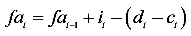 .
.