Open Journal of Marine Science
Vol.05 No.01(2015), Article ID:53215,14 pages
10.4236/ojms.2015.51010
An Assessment to Relationships between the Yellowfin Tuna and the Spotted Dolphin in Eastern Pacific Ocean (EPO) from 1998 to 2006
Gabriel Aldana Flores1,2, Juan Madrid Vera1*, Ana Quan Kiu Rascon3, Sergio G. Castillo Vargamachuca2, Ricardo Meraz Sanchez3
1Instituto Nacional de Pesca, CRIP Mazatlán, Sinaloa, México
2Posgrado en Ciencias Biológico Agropecuarias, Universidad Autónoma de Nayarit, Tepic, Mexico
3Posgrado en Ciencias del Mar y Limnología, Universidad Nacional Autónoma de México, Mexico City, Mexico
Email: Gabrielald2002@yahoo.com, *juanchomvera@yahoo.com.mx, anioux22@yahoo.com, rmeraz@ola.icmyl.unam.mx, arodriguez@ola.icmyl.unam.mx, sergio_machuca_@hotmail.com
Copyright © 2015 by authors and Scientific Research Publishing Inc.
This work is licensed under the Creative Commons Attribution International License (CC BY).
http://creativecommons.org/licenses/by/4.0/


Received 22 December 2014; accepted 8 January 2015; published 14 January 2015
ABSTRACT
Database belong to the Programa Nacional de Aprovechamiento del Atún y Protección de los Delfines (PNAAPD) from México. The area covers from latitude 5 to 20 N and longitude 90 to 125 W, Eastern Pacific Ocean (EPO), for 1998, 2001, 2002, 2005 and 2006 includes date, geographical position, sea surface temperature, tuna’s catch, yellowfin tuna’s size and dolphin’s number. 5 degress squares of latitude and longitude, each year were made. Yellowfin tuna number was normally distributed (KSd = 0.02, P > 0.20). The problem to solve is the relationship of the spotted dolphin and yellowfin tuna, that may analyze in the background of a non linear generalized model. Considering the array of latitude and longitude over the years that the abundance of yellowfin tuna is a dependent variable and the spotted dolphin abundance is the covariance continuous variable, the interaction and covariance, indicates a significant contribution to variability. The tuna abundance index does produce significative differences in latitude and longitude. Considering the dolphin as a dependent variable and the yellowfin tuna as a covariance continuous variable, the dolphin abundance index produced significative differences in latitude and longitude.
Keywords:
Yellowfin Tuna, Spotted Dolphin, North Pacific Ocean, Non Linear Generalized Model

1. Introduction
Considering nature, the first direct observation is diversity, biological communities, species assemblage or set of association, population is an abstraction, yet, obvious your existence. Different ideas about how communities use and share the same habitat, in this case, the pelagic zone, habitat in which both species, tuna and dolphin are feeding and gets protection. Factors such as sunlight and temperature favor survival for both species.
In general, yellowfin tuna has partnerships with various species like seabirds, dolphins and even sharks or whales [1] [2] , in case of dolphin’s species, it appears that environmental influence and therefore the association is modify according to the dolphin species and the geographic location.
In most cases, when species compete for similar resources it matches the same habitat and tends to divide the resource availability [3] ; causing the occupancy of different locations to hunt the same prey [3] - [5] . These strate- gies have been observed in a large numbers of taxa, including primates [6] [7] and carnivores [8] . Studies in the division of habitat and resources into small odontocetes are complicated due to the fact of difficulty of observation in open water [4] .
In the eastern Pacific Ocean (EPO), the dolphins are commonly associated with schools of yellowfin tuna. These polyspecific associations have been extensively studied over the tropical Pacific, [9] - [11] like tuna and other fish, marine mammals, seabirds and sharks [1] [12] .
These polyspecific aggregations, are integrated when social species creates feeding groups becoming very large, increasing success, avoiding threats from predators [1] [13] . These animals are known to feed, interact and move together for very long periods [11] . Feeding aggregations occur mainly in tropical waters, where the prey is carried to the surface, as their abundance and diversity allowing this species feed at the same time [10] [14] .
Each species seems to have preferred prey, but, has been shown that spotted dolphins are opportunistic and takes advantage for local and seasonal abundance of prey [1] [15] . It has been observed in the eastern Pacific Ocean (EPO) species of dolphins, which are the most common in the tuna-dolphin interaction spotted dolphin (Stenella attenuata), spinner dolphin (Stenella longirostris), common dolphin (Delphinus delphis), bottlenose dolphin (Tursiops truncatus) [16] [17] . For example, in the northwestern Atlantic, the common dolphin diet consists mainly of large fish like capelines (Mallotus villosus) and mackerel (Scomber scombrus) [18] [19] .
It is not well understood yet, the reasons for the strong link between yellowfin tuna and dolphins in the EPO, but this persistence and strength clearly indicates that at least one of these animals derives in some benefit from this polyspecific association [1] [11] [13] . Then is hard the explanation, in this work we advance a descriptive explanation, perhaps later we may work in other aspect, such as the relationships of sea-surface temperature, depth or herd structure.
The tuna-dolphin interaction is the main problem to solve, or at least, generating the most accurate scenario to explain how this works (or at least to create the most accurate scenario to explain this case). The starting point, supposed the population respect to geographical distribution in time, may help to generate hypotheses for this. We make this assumption through the abundance index analysis for both species respect to categorical arrangement of latitude and longitude, respect to years, and the temperature anomalies (for example, Figure 1).
So, the diverse works does emphasis in benefit result of this association, with support of course in their existence, the relationship between species, may be emphasized for that despite of tuna fishing, the dolphin’s number and the biomass is maintained, particularly the spotted dolphin, that may support also the effort of avoid damage or effect in dolphin population, that is necessarily continuous to enforce and enhancement.
2. Study Area
The Eastern Tropical Pacific Ocean (EPO) is defined as the area bounded by the coastline of the American con- tinent, the 40˚ North parallel, the 150˚ West meridian and the 40˚ South parallel. Is one of the most productive in the world’s tropical oceans. This area is characterized by the presence of highly migratory species such as tuna, billfish and sharks [20] . The thermal structure of the tropical Pacific is characterized by a mixing layer where the temperature is almost constant, a thermocline with a very strong heat exchange and a subsurface layer where intervals decreases lower than the thermocline [21] . The annual variation of surface temperature fluctuates be- tween 26˚C and 28˚C [22] . The intrusion of subtropical subsurface water promotes annual changes of 5˚C or more in the area near Cabo Corrientes, while in the Gulf of Tehuantepec between 3˚C and 4˚C. Warm water at Tropical Pacific are subject of a surface heating which tends to reduce the density, however, excessive evaporation which takes place in the subtropics, increases the density of surface and promotes convection and consequently a con-

Figure 1. Sea surface temperature anomalies data (˚C). The anomaly is produced from data haul or event register minus the average from these for the period from 1998 to 2006.
stant mixing process with a vertical extension of mixed layers of 20 to 50 meters.
According to the general circulation of the atmosphere, Mexico is between the south and anticyclonic zone of equatorial calms. The winds are generated in the southern anticyclonic, due to the rotation of the earth takes a SW direction and are present at the lower atmosphere, called trade winds, and on reaching the doldrums, is pro- duced an inversion and are directed towards north on the higher atmosphere down to the anticyclonic zone [23] [24] .
Then the region is under the influence of the California Current, North Equatorial Countercurrent, and Costa Rica’s dome [25] - [30] . The Tropical Eastern Pacific Ocean, is influenced of surface water in the central tropical. The edges north and south of the area are under the influence of subtropical surface waters. In the north, subtropical surface waters are present, made up warm surface water. The California Current appears as a mass of cold water, appearing in the winter [31] [32] . The influence of Costa Rica’s current expands to the tip of the Baja California peninsula and appear from August to December [27] [30] . This area is also under the influence of El Niño-Southern Oscillation [32] - [37] .
The Eastern Tropical Pacific Ocean contains some of the most productive waters in the world [20] . The upper levels of the pelagic food web include large tuna, dolphins, sharks, billfish and other species.
3. Materials and Methods
Used data from México dolphin tuna program (PNAAPD), for the years 1998, 2001, 2002, 2005 and 2006 include the date, the geographical position, the sea surface temperature, the tuna catch in ton, the mean size of yellowfin tuna [38] [39] , and the best estimation of dolphins made by the observer on board. Weight- length ratio [40] and the mean size were transformed in weight, later the tuna catch in numbers of yellowfin tuna.
Total of 1968 spotted dolphins in the data were analyzed. In a square of 5 degrees latitude and longitude, respect to the year, that content enough data or set hauls to replicate, were 45, 437, 725, 548 and 208 (Figure 2 and Figure 3). We define categorical variables for latitude and longitude using 5 degrees squares. In relation to data quality only is considering the study area from 5 latitude North (for example from 5 to 9 is the category 5, and successively) and 125 longitude West (from 125 to 129 is the category 125, and successively) (Figure 2 and Figure 3). These arrangements correspond only to the analyzed years.
Data from the tuna dolphin program and the years mentioned above were analyzed using a non linear generalized model, a factorial variance analysis was used as starting point. For the abundance index, we used the log of the number of yellow fin tuna and also the spotted dolphin as a dependent variable.
Using tuna’s number as a dependent variable, the covariate in model was the natural logarithm of the dol- phin’s number.
Using the dolphin’s number as a dependent variable, the covariate in model, was the natural logarithm of the number of tuna.
As a first analysis of the yellow fin tuna and spotted dolphn data distribution, were transformed to dispersion; data minus the mean. Also, number's natural log, or Ln y + 1, and the dispersion realted to Ln mean.
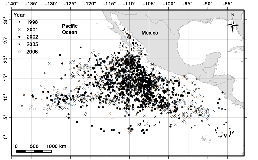
Figure 2. Dolphin sets made by the Mexican purse-seine fleet for the years 1998, 2001, 2002, 2005 and 2006 with yellowfin tuna positive catch.1**

Figure 3. Spotted dolphin abundance for sets analyzed and when there was positive yellowfin tuna catch, for the period from 1998 to 2006.1**
The problem to solve is the relationship between the spotted dolphin and yellow fin tuna. We suppose that the population number or the herd size respect to the geographical distribution in time, may help to generate hypo- theses to this population. Moreover produces basic information on the biology population, the fisheries and these species relations.
Maybe the problem analyzed by a variance analysis in the background of the non linear generalized model. Considering the matrix for latitude and longitude in categorical arrangement respect to year when the abundance for yellowfin tuna is a dependent variable and the spotted dolphin abundance is a covariance continuous variable. Also is possible, considering the dolphin as a dependent variable and the yellow fin tuna as a covariance conti- nuous variable.
The general linear model, the response variable y is linearly associated with values in the variable x as follows

When b0 is the intercept, bi is the regression coefficient; e is the error, cannot be explained by predictions; the expected value of e is assumed to be 0, while relations in the generalized nonlinear model is assumed by:

where e is the error, g (...) is a function, commonly the inverse function of g (...), and f (...) is called the link function, as:

where Uy is the explanation of the expected value of y. (See, e.g., [41] - [43] , various packages include analysis as Statistica and SPSS)
As an example of use of the inverse function, we should mention that the probability distribution F of a calculated value of the distribution, the associated probability given the degrees of freedom in the numerator and denominator, i.e. between the effect and error. The inverse of F is a probability value of F, which counts for the calculated number is the ratio of the mean square of treatment on the mean square error.
Several link functions can be chosen depending on the assumed distribution of the variable y as: Normal Distribution, Gamma, Inverse Normal, or Poisson. Normal distribution was used, and link function is the identity, reason why the tuna’s number in natural log is distributed as a normal.
In relation to dependent variable a linear generalized model, considering covariance in first place, the dolphin and in a second run the yellowfin tuna, that attempt to solve the main problem of this work.
The estimating parameters of the generalized linear model, from b0 to bk and the scale parameter, in the gene- ralized linear model are obtained by maximum likelihood (ML) estimation, through iterative procedures. The iterative methods for ML estimation in the generalized linear model, of which the Newton-Raphson and Fisher-Scor- ing methods are efficient and widely used [44] [45] . The Fisher re-weighted least squares method for example pro- vides for all generalized linear models, also provides a variance-covariance matrix for estimating parameters as a product of its calculus [45] .
The sums of squares involve a partitioning of the whole model. The sums of squares provide a complete de- composition of the predicted sums of squares for the whole model.
Some test may compare the prediction respect to observed mean for the matrix arrangement, showing only the raw and studentized residual.
4. Results
We analyze 1968 spotted dolphin sets (Figure 3). The data were arranged in a square of 5 degrees of latitude and longitude, respect to each year. For example, from 5 Latitude North and from 90 to 125 Longitude West, there are 471 replicates or sets, for 10 Latitude North and from 90 to 125 Longitude West includes a 432 sets, for 15 Latitude North and from 90 to 125 Longitude West includes a 551 sets and for 20 Latitude North and from 90 to 125 Longitude West includes a 426 sets. Per year were, in 1998, 179 sets; in 2001, 521 replicates; in 2002, 410; in 2005, 407, and in 2006, 426 replicates or sets (Figure 2 and Figure 3).
The distribution of data analysis is shown in Figure 4. Comparing the data for yellowfin tuna and the spotted dolphin, the distribution is represented for the percentage and accumulated percentage of solution produced by a normal fitting.

Figure 4. An analysis of the data distribution for yellowfin tuna and the spotted dolphin. The distribution represents the percentage and cumultive percentage of solution produced for a normal fitting. The tuna data may be fitted by a normal. The dolphin data contains a portion of the zero register as shown in the figure. The data is used in natural log.
The tuna’s data may be fitted by a normal distribution, using the natural log data and Kolmogorov Smirnov d = 0.018 and p is non-significative, therefore rejects the null hypotheses that the data distribution is not different to a normal (Figure 4). The dolphin data contains a portion of the zero register as it’s shown in Figure 4, but is susceptible of explanations in Normal theory, and for that the non linear model not as a necessary condition.
We ran the non linear model for the yellowfin tuna log number, as a dependent variable, respect to the cate- gorical arrangement for the latitude and longitude and the years. The natural log of the spotted dolphin is a co- variate variable. Using a sigma restricted parameterization, and Likelihood Type test.
In Table 1, left table, shows the results for the model. The abundance index or natural log of the spotted dol- phin produces a significative effect in the variance of the model, in this case in the abundance index for the yel- lowfin tuna. Moreover there are significative effects for the years and latitude. It seems an effect on the interaction of latitude and year. Meaning an interaction of latitude and the interaction of latitude respect to years analyzed.
In fisheries data context, the effects or differences of the index in the longitude and the interaction in longi- tude and years also may be take in count (Table 1, left part), consider that near to 80% of the variance may be explained (p < 0.193 by the interaction for example).
In Table 1, right table, shows the results for the model. The abundance index or natural log of the yellowfin tuna produces a significative effect in the variance of the model, in this case in the abundance index for the spotted dolphin. There are significative effects or differences for the years, latitude and longitude. Apparently also there are effect for the interaction in latitude and years and longitude and years. Apparently, there are effects on the interaction in latitude/years and longitude/years, interaction effects exists on latitude and latitude/ years.
Figure 5 shows the abundances index and their 95% confidence interval, for the tuna and dolphin data. At the top part, there are two graphs for the years (a, d), in the middle part there are two graphs for the latitudes (b, e) and in the lower part two graphs for the longitudes (c, f). The abundance indexes for both species were significa- tive different for years. For the latitudes both species produces significative differences. Dolphin’s abundance index was significative for longitude.
In Figure 5(a), abundances index and their confidence interval of 95%, for the tuna is decreasing from 1998 to 2006 and dolphin data increase from 1998 to a maximum in 2001 and slightly changes to 2006 (Figure 5(d)). The middle part, center Figure 5(b), shows clear differences with a maximal in 20 North for the abundance index

Figure 5. The abundances index and their confidence interval of 95%, for the tuna (left part) and dolphin data (right part). The first row (a) represented in Ln of yellow fin tuna and dolphins (Part (d)) vs. years. Second row, represented in Ln of yellow fin tuna and dolphins (Part (e)) vs. latitude. Third row represented in Ln of yellow fin tuna and dolphins (Part (f)) vs. longitude.

Table 1. Results for the non-linear generalized model. The index of abundances or natural log for the sppotted dolphin produces a significative effect in variance’s model; the abundances index of the yellowfin tuna (left part). The right part, the abundances index or natural log for the yellowfin tuna produces significative effect in variance’s model, in the abundances index of the sppotted dolphin. The results shows a significative effect on the interaction of latitude and longitude respect of the years analyzed. D.F. Degrees of freedom.
of the yellowfin tuna, and a conspicuous descending for the dolphin’s abundances index in 20 North (Figure 5(e)). For the longitude in the inferior part of Figure 5(c), the dolphin was signficative in abundance index, shown two dolphin’s population, that have a cross over in 110 W. If we use longitude as a category, the mean of yellowfin tuna number, it may be say is more homogeneous.
The interaction for abundance index of both species in latitude and year is shown in Figure 6. This index for the yellowfin tuna using latitude and year do not produces differences (Table 1, Figure 6(a)).The same index for dolphins using latitude and year produces differences (Table 1, Figure 6(b)).
The interaction for abundance index or Ln yellow tuna number for latitude and year produce differences (Year × Latitude (Table 1)). The major abundances were observed in 20 North, from 1998 to 2006 (Figure 6, part a 20 N). The next in order, was 5 North in 1998 and 2001, latitude in which is observed the lowest abun- dance in 2005, but in 2006 are recovering. In the latitude 10 and 15 North the values fluctuates around the 5 and 20 North, in 2006 year both values are the lowest (Figure 6(a); 5 N).
The interaction of the dolphin abundance index for latitude and year also produces significant differences. The major abundances were observed in 5 North, from 1998 to 2006. In general, its observed a gradient descent from latitude 5 to 20 North (Figure 6(b)) (a gradient descent is observed*). The lowest abundance index value is observed in latitude 20 North, from 1998 to 2006.
Figure 7 shows the arrangement of the interaction abundance index of both species in latitude, longitude and year that produces differences for the tuna and dolphin, in separated analysis. The figure represents both species only for practical comparisons.
The index of interaction for the yellowfin tuna abundances respect to the latitude, longitude and years produce significative differences (Table 1, Year × Latitude × Longitude, Figure 7). The abundances were major in 1998 and descend the next years, if following the abscissas magnitude. 2005 is an exception, where there is an increase at 10 North.
In general, the interaction of abundances for yellowfin tuna may indicates the general stability of these indexes among the latitude and longitude but there are changes among the years.
 (a)
(a) (b)
(b)
Figure 6. The index of abundances and latitude interaction. Top part of the graph for tuna (a) and bottom part for dolphins (b).

Figure 7. Index of interaction of spotted dolphin and tuna abundances respect to the latitude, longitude and years. Both interactions contributes in a significative way to the model.
Figure 7 shows the interaction index for spotted dolphins abundance respect to latitude, longitude and years (left part), interaction that contribute in a significative way to the model. The abundance index increases in 1998, a maximum in 2001 and slightly changes in towards 2006. A small decrease for dolphin’s abundance index is at 20 North. According to longitude, maybe was analyzed two different dolphin’s population, this assumption due to the result that have a confluence in 100 W, conspicuous in 2001, 2005 and 2006.
In general, the interaction of abundances for the spotted dolphin may indicate the general variability of these along the latitude, the longitude and years. The variability in marine mammals populations sizes is greater, than the fish ones, when consider the longitude for example.
Figure 8 shows, the error for the index of abundances for the yellowfin tuna and spotted dolphin respect to the latitude, longitude and years in raw and prediction by studentized residual. There is a relative distribution around zero, the log distribution explains the positive skeweed related to catch searching for positive catch. The observed data and prediction in general is explained for the arrangement, the difficulties are the explanation about the relative signficances. The errors show the verisimilitude of the model; by product that the natural lo- garithm of yellowfin tuna’s index do not produces differences respect to a normal distribution. However, we used the model as a heuristic tool to explain this relationship.
5. Discussion
The database analyzed in this work was provided by the Programa Nacional de Aprovechamiento del Atún y Protección de los Delfines (PNAAPD), made up by fishing sets with date, geographical position, sea-surface temperature, number of cruise, tuna catch in tons, tuna’s sizes, dolphin’s species, dolphin’s number of first and second estimate made by observer on board, and number of animals from four species of dolphins. From this database we analyzed a total of 1968 sets associated to marine mammals (LANMAM), taking the best estimate dolphin’s number for the abundances of dolphin’s species when also was recorded of the size of yellowfin tuna [38] . The capture zone of yellowfin tuna has shown certain patterns in the OPO fishing areas [39] [46] . We analyzed the years 1998, 2001, 2002, 2005 and 2006, which included periods of normal weather, a period of cold and warm anomalies as La Niña or El Niño, known as El Niño/Southern Oscillation (ENSO) and covered a period which may include a decadal variation, linked to the Kurishio’s circulation system. Data, periods and covered area can support the consideration that contained enough information to analyze the interaction of tuna and dolphins (Figure 2).
A first approach, which has already been attempted in classical works of the subject [12] [13] [47] -[59] inter- prets basic descriptive information, the central tendencies and dispersion of data.
In the case that tuna-dolphin’s interaction was thought, until recent years that the most likely explanation of this relationship was that dolphins possess a greater ability to find food that tuna because of its ability to echo- locate, these arguments have been formulated based on energy and mathematical models, as well as potential advantages in food [60] - [62] , but only the diet of tuna and spotted dolphin registered in matches [53] [63] [64] .
Partnerships (the association) consist of all these (consist in the fact that all these) species as (ARE) common predators in tropical waters of the Eastern Pacific ocean, and as a positive correlation between dolphins herd, tuna schools and their interaction with the ecosystem [10] [65] [64] .

Figure 8. The abundance index’s error for the yellow fin tuna and spotted dolphin respect to the latitude, longitude and years in a prediction by studentized residual. There is a relative distribution around zero, the log distribution explains the positive skeweed related to searching and positive catch.
A review of the same data [66] , observed that the purse seine fleet first sights the dolphins HERDS, based on the knowledge that tuna’s school associated to dolphin’s herds are bigger sizes; therefore these are the sets con- ducted by the fleet. Considering this as a type of operational interaction, related to the probability of obtaining bigger catches and larger sizes. The results obtained for this interaction was, tuna associated to mix herds of spotted dolphins and eastern spinner dolphins reaches the highest probability (50% of the mean); then, followed by the tuna associated to spotted dolphins herds. Third, tuna associated to mixed herds of spotted dolphins, eastern spinner and white belly spinner. [66] mentioned that spotted dolphin herds has a variable number from 100 to 1000 individuals, with an equatorial distribution, not beyond 10 North, after this longitude, the herd starts to decrease in number, while longitudinally the largest herd are not beyond 115 W. Most of the sights are far from the coastline but their number is smaller (up to 500 individuals). Mean while the temperature anomalies plays an important role for the spotted dolphin in their distribution, showing in the analysis that are related to latitude, longitude and the year, this may explain the distribution in subtropical and tropical waters, in addition to the tropic relationships and the abundance of food resources.
In the analyzes this study shows that the distribution of dolphin species is related to the latitudinal distribution and this is to emphasize the distribution of water masses and ocean currents (California Current, North Equatorial Current, Undertow North Equatorial and the Costa Rica Dome) of which several have advanced in this work [24] [50] [67] [68] . For the herds, the longitude plays an important role only when taking into account their size and its association with tuna school’s size, probably to the distance far from the coast to cover a larger area in a larger herd, increases the chances of success in food, and the association with tuna is higher, therefore the largest catches were recorded those years; the strength of this interaction clearly indicates that at least one of the parts drives on some benefit from this polyspecific association [1] [11] [13] [14] [69] , by linking the presence with dolphin species the tuna catch was the largest, in sizes and weight while it was associated with the spotted dolphin, 49% chance [66] (Figure 3) and although, this value decreases according to the number of species pre- sent, if there is a strong association for the sets associated with dolphins.
[64] [70] - [72] reported that dolphin species that form herds of hundreds or thousands, typically live in pelagic habitats where it is believed that predation pressure should be higher, while coastal and shallow species are typi- cally smaller, therefore the tuna’s size will also depend on the school's size that is associated to. [68] [73] - [75] , reported that herds of spotted dolphin, eastern spinner and white belly spinner are mostly found in areas far from the coast, matching with the largest sizes of schools associated with the largest herds of species mentioned above.
The abundance of biomass is associated with fluctuations in phytoplankton and zooplankton and the intensity of El Niño [76] [77] , although, in most of the cases the temperature has some influence, in this case, the spotted and spinner dolphin with two sub species seems to move together or similar, being the main factor related to the latitude related to the latitude, this influence is shown at the factorial design and in second degree of influence, will be the longitude, considering the latitudinal distribution does show an important influence. For example for the common dolphin, longitudinal location acts as if the temperature was a determining factor.
It has been observed that yellow fin tuna interacts with various species such as sea birds, dolphins and shark or whales [1] [2] ; dolphin’s species are influenced by the environment and therefore this association will be modified by the species related and geographical location of each set done by the purse seine fleet.
Acknowledgements
To the National Fisheries Bureau in Mexico (National Fisheries Institute of Mexico) (Instituto Nacional de Pesca). To Programa Nacional de Aprovechamiento del Atún y Protección de los Delfines (PNAAPD) for the database used. To CONACYT for the financial support given to the last authors during their masters and doctoral studies.
References
- Das, K., Lepoint, G., Loizeauà, V., Debacker, V., Dauby, P. and Bouquegneau, J.M. (2000) Tuna and Dolphin Associations in the North-East Atlantic: Evidence of Different Ecological Niches from Stable Isotope and Heavy Metal Measurements. Marine Pollution Bulletin, 40, 102-109. http://dx.doi.org/10.1016/S0025-326X(99)00178-2
- Rogan, E. and Mackey, M. (2007) Megafauna Bycatch in Drift Nets of Albacore Tuna in the NE Atlantic. Fisheries Research, 86, 6-14. http://dx.doi.org/10.1016/j.fishres.2007.02.013
- Roughgarden, J. (1976) Resource Partitioning among Competing Species: A Coevolutionary Approach. Theoretical Population Biology, 9, 388-424. http://dx.doi.org/10.1016/0040-5809(76)90054-X
- Bearzi, M. (2005) Dolphin Sympatric Ecology. Marine Biology Research, 1, 165-175. http://dx.doi.org/10.1080/17451000510019132
- Begon, M., Townsend, C.R. and Harper, J.L. (2006) Ecology. From Individuals to Ecosystems. Blackwell Publishing, Oxford.
- Tutin, C.E.G. and Fernández, M. (1984) Nationwide Census of Gorilla (Gorilla g. gorilla) and Chimpanzee (Pan t. tro- glodytes) Populations in Gabon. American Journal of Primatology, 6, 313-336. http://dx.doi.org/10.1002/ajp.1350060403
- Kuroda, S., Nishihara, T., Suzuki, S. and Oko, R. (1996) Sympatric Chimpanzees and Gorillas in the Ndoki Forest, Congo. In: McGrew, W.C., Marchant, L.F. and Nishida, T., Eds., Great Ape Societie, Cambridge University Press, Cam- bridge, 71-81. http://dx.doi.org/10.1017/CBO9780511752414.008
- Wu, H.Y. (1999) Is There Current Competition between Sympatric Siberian Weasels (Mustela sibirica) and Ferret Bad- gers (Melogale moschata) in a Subtropical Forest Ecosystem of Taiwan? Zoological Studies, 38, 443-451.
- Perrin, W.F., Warner, R.R., Fiscus, C.H. and Holts, D.B. (1973) Stomach Contents of Porpoise, Stenella spp., and Yel- low Fin Tuna, Thunnus albacares, in Mixed-Species Aggregations. Fishery Bulletin, 71, 1077-1092.
- Au, D.W. and Pitman, R.L. (1986) Seabird Interactions with Dolphins and Tuna in the Eastern Tropical Pacific. The Condor, 88, 304-317. http://dx.doi.org/10.2307/1368877
- Au, D.W. (1991) Polyspecific Nature of Tuna Schools: Shark, Dolphin and Seabird Associates. Fishery Bulletin, 89, 343-354.
- Gerrodette, T. and Forcada, J. (2005) Non-Recovery of Two Spotted and Spinner Dolphin Populations in the Eastern Tropical Pacific Ocean. Marine Ecology Progress Series, 291, 1-21. http://dx.doi.org/10.3354/meps291001
- Scott, M.D. and Cattanach, K.L. (1998) Diel Patterns in Aggregations of Pelagic Dolphins and Tunas in the Eastern Pacific. Marine Mammal Science, 14, 401-428.
- Heithaus, M.R. (2001) Predator-Prey and Competitive Interactions between Sharks (Order Selachii) and Dolphins (Suborder Odontoceti): A Review. Journal of Zoology, 253, 53-68. http://dx.doi.org/10.1017/S0952836901000061
- Wurtz, M. and Marrale, D. (1993) Food of Striped Dolphin, Stenella coeruleoalba, in the Ligurian Sea. Journal of the Marine Biological Association of UK, 73, 571-578. http://dx.doi.org/10.1017/S0025315400033117
- Lennert-Cody, C.E. and Scott, M. (2005) Spotted Dolphin Evasive Response in Relation of Fishing Effort. Marine Mammal Science, 21, 13-28. http://dx.doi.org/10.1111/j.1748-7692.2005.tb01205.x
- Wade, P.R., Watters, G.M., Gerrodette, T. and Reilly, S.B. (2007) Depletion of Spotted and Spinner Dolphins in the Eastern Spinner Dolphins in the Eastern Tropical Pacific: Modeling Hypotheses for Their Lack of Recovery. Marine Ecology Progress Series, 343, 1-14. http://dx.doi.org/10.3354/meps07069
- Overholtz, W.J. and Waring, G.T. (1991) Diet Composition of Pilot Whales Globicephala sp. and Common Dolphins Delphinus delphis in the Mid-Atlantic Bight during Spring 1989. Fishery Bulletin, 89, 723-728.
- Ostrom, P.H., Lien, J. and Macko, S.A. (1993) Evaluation of the Diet of Sowerby’s Beaked Whale, Mesoplodon bidens, Based on Isotopic Comparisons among North-Western Atlantic cetaceans. Canadian Journal of Zoology, 71, 858-861. http://dx.doi.org/10.1139/z93-110
- Barber, R.T. and Chávez, F.P. (1986) Ocean Variability in Relation to Living Resources during the 1982/83 El Niño. Nature, 319, 279-285. http://dx.doi.org/10.1038/319279a0
- Tchernia, P. (1980) Descriptive Regional Oceanography. Pergamon Press, Nueva York.
- Shea, D.J., Trenberth, K.E. and Reynolds, R.W. (1992) A Global Monthly Sea Surface Temperature Climatology. Journal of Climate, 5, 987-1001. http://dx.doi.org/10.1175/1520-0442(1992)005<0987:AGMSST>2.0.CO;2
- Tamayo, J.L. (1984) Geografía Moderna de México. Trillas, México.
- Trasviña, A. and Barton, E.D. (2008) Summer Circulation in the Mexican Tropical Pacific. Deep Sea Research Part I: Oceanographic Research Papers, 55, 587-607. http://dx.doi.org/10.1016/j.dsr.2008.02.002
- Wyrtki, K. (1965) Surface Currents of the Eastern Tropical Pacific Ocean. Bulletin Inter-American Tropical Tuna Commission, 9, 269-304.
- Garfield, P.C., Packard, T.T., Friederich, O.E. and Codispoti, L.A. (1983) A Subsurface Particle Maximum Layer and Enhanced Microbial Activity in the Secondary Nitrite Maximum of North-Eastern Tropical Pacific Ocean. Journal Marine Research, 41, 747-768. http://dx.doi.org/10.1357/002224083788520496
- Baumgartner, R.T. and Christensen, N.J. (1985) Coupling of the Gulf of California to Large-Scale Interannual Climatic Variability. Journal of Marine Research, 43, 825-848. http://dx.doi.org/10.1357/002224085788453967
- de la Lanza, G. (1991) Oceanografía de mares mexicanos. AGT Editor, México.
- Xie, L. and Hsieh, W.W. (1995) The Global Distribution of Wind-Induced Upwelling. Fisheries Oceanography, 4, 52- 67. http://dx.doi.org/10.1111/j.1365-2419.1995.tb00060.x
- Badan, A. (1997) La Corriente Costera de Costa Rica en el Pacífico Mexicano. In: Lavin, F.M., Ed., Contribuciones a la Oceanografía Física en México, Unión Geofísica Mexicana, Mexico, 99-113.
- Fiedler, C.P. (1992) Seasonal Climatologies and Variability of Eastern Tropical Pacific Surface Waters. NOAA Technical Report NMFS, 108, 109.
- Fiedler, P.C., Chavez, D.W. and Behringer, S.B. (1992) Physical and Biological Effects of Los Niños in the Eastern Tropical Pacific, 1986-1989. Deep Sea Research Part A. Oceanographic Research Papers, 39, 199-219. http://dx.doi.org/10.1016/0198-0149(92)90105-3
- Ramp, S.R., McClean, J.L., Collins, C.A., Semter, A.J. and Hays, K.A.S. (1997) Observations and Modeling of the 1991-1992, El Niño Signal off Central California. Journal of Geophysical Research: Oceans, 102, 5553-5582. http://dx.doi.org/10.1029/96JC03050
- Madrid-Vera, J. and Sánchez, P. (1997) Patterns in Marine Fish Communities as Shown by Artisanal Fisheries Data on the Shelf off the Nexpa River, Michoacán, Mexico. Fisheries Research, 33, 149-158. http://dx.doi.org/10.1016/S0165-7836(97)00059-3
- CIFEN (2006) El Niño/La Niña: La Perspectiva en el Pacífico Oriental. Centro Internacional para la Investigación del Fenómeno El Niño. http://www.ciifen-int.org/
- NOAA (2007) Tropics. Climate Diagnostic Bulletin, National Oceanic and Atmospheric Administration. http://www.cpc.ncep.noaa.gov/products/analysis_monitoring/bulletin_1206
- NOAA (2012) El Niño/Southern Oscillation (ENSO) Diagnostic Discussion. Diagnostica emitido por centro de predic- ciones climaticas/ncep/nws y el Instituto Internacional de Investigación de clima y sociedad. Traducción cortesía de: Wfo san juan, puerto rico. http://www.cpc.ncep.noaa.gov/products/analysis_monitoring/enso_advisory/
- Solana-Sansores, R., Aldana, F.G. and Compeán, J.G. (2001) Muestreo a bordo de barcos mexicanos para estimar la estructura poblacional del atún aleta amarilla (Thunnus albacares) del Pacífico Oriental. Hidrobiologica, 11, 123-132.
- Aldana, G. (2000) Análisis por tipo de lance de las frecuencias de longitudes del atún aleta amarilla (Thunnus al- bacares, Bonaterre, 1865), obtenidas mediante un diseño de muestreo probabilístico a bordo de barcos cerqueros mexi- canos. Tesis, Universidad Autónoma de Nuevo León, México.
- Zhu, G., Xu, L., Zhou, Y. and Dai, X. (2008) Length-Frequency Compositions and Weight-Length Relations for Big Eye Tuna, Yellow Fin Tuna, and Albacore (Perciformes: Scombrinae) in the Atlantic, Indian, and Eastern Pacific Ocean. Acta Ichthyologica Et Piscatoria, 38, 157-161. http://dx.doi.org/10.3750/AIP2008.38.2.12
- Montgomery, C.D. (1991) Design and Analysis of Experiments. John Wiley and Sons, Hoboken.
- Lyman, M.O. (1993) An Introduction to Statistical Methods and Data Analysis. Duxbury Press, Belmont.
- Quinn, G.P. and Keough, M.J. (2002) Experimental Design and Data Analysis for Biologist. Cambridge University Press, Cambridge. http://dx.doi.org/10.1017/CBO9780511806384
- Dobson, A.J. (1990) An Introduction to Generalized Linear Models. McGraw-Hill, New York.
- Stat Soft Inc. (2004) STATISTICA (Data Analysis Software System). Version 7. www.statsoft.com
- CIAT (2008) Reporte de la Comisión Interamericana del Atún Tropical. La Jolla.
- Mitchell, E. (1975) Porpoise, Dolphin and Small Whale. Fisheries of the World. Status and Problems. International Union for Conservation of Nature and Natural Resources (IUCN), Morges.
- Northridge, S.P. (1984) World Review of Interactions between Marine Mammals and Fisheries. FAO Fisheries Technical Paper 251, Food and Agriculture Organization of the United Nations, Rome.
- Northridge, S.P. and Hoffman, R.J. (1999) Marine Mammal Interaction with Fisheries. In: Twiss, J.R. and Reeves, R.R., Eds., Conservation and Management of Marine Mammals, Smithsonian Institution, Washington & London, 99- 119.
- Reilly, S.B. (1990) Seasonal Changes in Distribution and Habitat Differences among Dolphins in the Eastern Tropical Pacific. Marine Ecology Progress Series, 66, 1-11. http://dx.doi.org/10.3354/meps066001
- Fiedler, P.C. and Reilly, S.B. (1994) Interannual Variability of Dolphin Habitats in the Eastern Tropical Pacific. 11: Effects on Abundances Estimated from Tuna Vessel Sightings, 1975-1990. Fishery Bulletin, 92, 451-463.
- Caddya, J.F. and Majkowski, J. (1996) Tuna and Trees: A Reflection on a Long-Term Perspective for Tuna Fishing around Floating Logs. Fisheries Research, 25, 369-376. http://dx.doi.org/10.1016/0165-7836(95)00449-1
- Finneran, J.J., Oliver, C.H.W., Schaefer, K.M. and Ridgway, S.H. (2000) Source Levels and Estimated Yellow Fin Tuna (Thunnus albacares) Detection Ranges for Dolphin Jaw Pops, Breaches, and Tail Slaps. Journal of the Acoustical Society of America, 107, 649-656. http://dx.doi.org/10.1121/1.428330
- Schaefer, K.M. and Oliver, C.W. (2000) Shape, Volume and Resonance Frequency of the Swimbladder of Yellow Fin Tuna (Thunnus albacares). Fishery Bulletin, 98, 364-374.
- Bearzi, G. (2002) Interactions between Cetacean and Fisheries in the Mediterranean Sea. In: Notarbartolo di Sciara, G., Ed., Cetaceans of the Mediterranean and Black Seas: State of Knowledge and Conservation Strategies, Section 9, A Report to the ACCOBAMS Secretariat, Monaco, Section 9, 20 p.
- Edwards, E.F. (2002) Energetics Consequences of Chase by Tuna Purse-Seiners for Spotted Dolphins (Stenella attenuata) in the Eastern Tropical Pacific Ocean. Southwest Fisheries Science Center National Marine Fisheries Service, NOAA (2002) Adminstrative Report LJ-02-29, p. 33.
- Enríquez-Andráde, R. and Vaca-Rodríguez, J.G. (2004) Evaluating Ecological Tradeoffs in Fisheries Management: A Study Case for the Yellow Fin Tuna Fishery in the Eastern Pacific Ocean. Ecological Economics, 48, 303-315. http://dx.doi.org/10.1016/j.ecolecon.2003.09.009
- Hoyle, D. and Maunder, M.N. (2004) A Bayesian Integrated Population Dynamics Model to Analyze Data for Protected Species. Animal Biodiversity and Conservation, 27, 247-266.
- Cramer, K.L., Perryman, W.L. and Gerrodette, T. (2008) Declines in Reproductive Output in Two Dolphin Populations Depleted by the Yellow Fin Tuna Purse Seine Fishery. Marine Ecology Progress Series, 369, 273-285. http://dx.doi.org/10.3354/meps07606
- Mullen, A.J. (1984) Autonomic Tuning of a Two Predator, One Prey System via Commensalism. Mathematical Biosciences, 72, 1-81.
- Edwards, F. (1992) Energetics of Associated Tunas and Dolphins in the Eastern Tropical Pacific Ocean: A Basis for the Bond. Fishery Bulletin, 90, 678-690.
- Wûrsig, B., Wellasn, R.S. and Norris, D.K.S. (1994) Food and Feeding. In: Norris, K., Wursig, B., Wellsy, R. and Wur- sig, M., Eds, The Hawaiian Spinner Dolphin, University of California Press, Berkeley, 216-231.
- INE (Instituto Nacional de Ecología) (2005) Fecha de última actualización: 29/08/2005. www.ine.gob.mx
- Hunsicker, M.E., Olson, R.J., Essington, T.E., Maunder, M.N., Duffy, L.M. and Kitchell, J.F. (2012) Potential for Top-Down Control on Tropical Tunas Based on Size Structure of Predator―Prey Interactions. Marine Ecology Pro- gress Series, 445, 263-277. http://dx.doi.org/10.3354/meps09494
- Au, D.W.K. and Pitman, R.L. (1988) Seabird Relationships with Tropical Tunas and Dolphins. In: Burger, J., Ed., Sea- birds and Other Marine Vertebrates: Competition, Predation and Other Interactions, Columbia University Press, New York, 174-212.
- Quan-Kiu, A.C. (2010) Análisis de las estructuras de tallas del atún aleta amarilla (Thunnus albacares) con respecto al tipo y tamaño de las manadas de delfines y las variaciones del medio ambiente en el Océano Pacífico Oriental. Tesis Maestría, Posgrado en Ciencias del Mar y Limnología, UNAM, México.
- Au, D.W.K. and Perriman, W.L. (1985) Dolphin Habitats in the Eastern Tropical Pacific. Fishery Bulletin, 83, 623- 643.
- Ballance, L.T., Pitman, R.L. and Fiedler, P.C. (2006) Oceanographic Influences on Seabirds and Cetaceans of the East- ern Tropical Pacific: A Review. Progress in Oceanography, 69, 360-390. http://dx.doi.org/10.1016/j.pocean.2006.03.013
- Stensland, E., Angerbjörn, A. and Berggren, P. (2003) Mixed Species Groups in Mammals. Mammal Review, 33, 205- 223. http://dx.doi.org/10.1046/j.1365-2907.2003.00022.x
- Norris, K.S. and Dohl, T.P. (1980) The Structure and Function of Cetacean Schools. In: Herman, L., Ed., Cetacean Behavior: Mechanisms and Functions, John Wiley & Sons, New York, 211-261.
- Wells, R.S., Irvinean, A.B. and Scott, D.M. (1980) The Social Ecology of Inshore Odontocetes. In: Herman, L., Ed., Cetacean Behavior: Mechanisms and Functions, John Wiley & Sons, New York, 263-317.
- Scott, M.D. and Chivers, S.J. (1990) Distribution and Herd Structure of Bottlenose Dolphins in the Eastern Tropical Pacific Ocean. In: Leatherwood, S. and Reeves, R., Eds., The Bottlenose Dolphin, Academic Press, San Diego, 387- 402. http://dx.doi.org/10.1016/B978-0-12-440280-5.50026-3
- Benoit-Bird, A. and Au, W.W.L. (2009) Cooperative Prey Herding by the Pelagic Dolphin, Stenella longirostris. Jour- nal of the Acoustical Society of America, 125, 125-137. http://dx.doi.org/10.1121/1.2967480
- Palacios, D.M. (2003) Oceanographic Conditions around the Galápagos Archipelago and Their Influence on Cetacean Community Structure. Ph.D. Thesis, Oregon State University, Corvallis.
- Perrin, W.F. and Hohn, A.A. (1994) Pantropical Spotted Dolphin―Stenella attenuata. In: Ridgway, S.H. and Harrison, S.R., Eds., Handbook of Marine Mammals, Academic Press, London, 71-98.
- Fiedler, P.C. (2002) Environmental Change in the Eastern Tropical Pacific Ocean: Review on ENSO and Decadal Variability. Administrative Report LJ-02-16. NOAA, Southwest Fisheries Science Center, La Jolla.
- Hampton, J.P., Kleiber, A., Langley, A. and Hiramatsu, K. (2004) Stock Assessment of Yellow Fin Tuna in the Western and Central Pacific Ocean. 17th Meeting of the Standing Committee on Tuna and Billfish SCTB17 Working Paper SA-1, Majuro, 9-18 August 2004, 74 p.
NOTES

*Corresponding author.

1Only as reference of similarity, spotted dolphin is the most common dolphin specie associated to yellowfin tuna’s catch. That is why both Figure 2 and Figure 3 look at first sight the same. First one (Figure 2) shows only the positive catch of yellowfin tuna during the period of study while Figure 3 (second one) shows the sights of spotted dolphins when there was positive catch of yellow fin tuna.