Open Journal of Statistics
Vol.4 No.5(2014), Article
ID:49087,16
pages
DOI:10.4236/ojs.2014.45041
Multivariate Modality Inference Using Gaussian Kernel
Yansong Cheng1, Surajit Ray2
1Quantitative Science, GlaxoSmithKline, King of Prussia, PA, USA
2School of Mathematics and Statistics, Glasgow University, Glasgow, UK
Email: yansong.x.cheng@gsk.com, surajit.ray@glasgow.ac.uk
Copyright © 2014 by authors and Scientific Research Publishing Inc.
This work is licensed under the Creative Commons Attribution International License (CC BY).
http://creativecommons.org/licenses/by/4.0/


Received 27 June 2014; revised 1 August 2014; accepted 10 August 2014
Abstract
The number of modes (also known as modality) of a kernel density estimator (KDE) draws lots of interests and is important in practice. In this paper, we develop an inference framework on the modality of a KDE under multivariate setting using Gaussian kernel. We applied the modal clustering method proposed by [1] for mode hunting. A test statistic and its asymptotic distribution are derived to assess the significance of each mode. The inference procedure is applied on both simulated and real data sets.
Keywords
Modality, Kernel Density Estimate, Mode, Clustering

1. Introduction
Mode is defined as the local maximum of a probability density. Modality, which is the number of the modes, is an important feature of any probability distribution. The natural evolution of multimodality occurs when a distribution is composed by several sub-populations. In practice, it is important to learn how many sub-populations the data have. In general, there are three different, but related, research areas that address this question: 1) the inference on the number of components in the finite mixture model; 2) estimating the number of clusters and/or merging the clusters of a clustering output; and 3) the modality inference. Each of these three approaches addresses the question of how many components the data have from its own angle. For the inference on the number of components in the mixture distribution, the hypothesis is usually
 versus
 where K is the parameter of the number of components. The likelihood ratio test (LRT) is often used to assess the significance of the hypothesis. However, in general, the distribution of the LRT is very complicated. More details can be found in e.g. [2] . Depending on the clustering method, the inference procedures on the number of clusters could be different. [3] proposed the GAP statistic, which contains information regarding the distance between the data points within each cluster. In particular, the authors applied the method on the K-means clustering [4] . [5] proposed the EM-clustering method, a model-based clustering method. The authors selected the ideal number of clusters by using the Bayesian information criterion (BIC), which is a model selection tool. However, as it is well established, BIC does not follow the regularity conditions and is inappropriate to use in the problem of determining the number of components.
The modality inference, which is used to assess the number of modes of the data, is often a robust nonparametric approach. There is a lot of existing literatures that address the problem of the modality of univariate probability distribution. These methods can be classified as the test of unimodality, bimodality or multimodality. Alternatively, these methods can be grouped as a global or local test. The global test considers the modality of the entire distribution. In contrast, the local test focuses on the specific region of the density that contains the particular investigated mode instead of considering the entire distribution.
In the case of the global test, [6] proposed the most commonly used critical bandwidth parameter, the smallest value of the bandwidth parameter h for which the KDE with Gaussian kernel
 (1.1)
(1.1)
is k-modal, where
 is the probability distribution function (pdf) of the standard normal distribution. To assess the significance, [6] suggested using
 as the bandwidth parameter, denoted as
 , and using the nonparametric bootstrap method proposed by [7] to sample the reference data, consequently to get the distribution of the test statistic under the null hypothesis.
Among the local tests, the one proposed by [8] is widely used. Denoting the mode as
 and the saddle point
 , the test statistic is defined as:

where i is the ith investigated mode and
 is the KDE in (1.1). It can be thought as the probability mass of the mode above the higher of the two saddle points or antimodes around it. The advantage of this statistic is that it does consider not only the heights of the mode and saddle point, but also the distance between them. The reference distribution is generated by forcing the distribution flat (uniform) between the point
 and
and
 and keeping the rest of the distribution the same.
The generalization to multivariate data is sparse. [9] proposed a mode hunting tool together with a further test of the significance for the existence of these modes, by using the k-nearest neighbor (KNN) density estimate for multivariate data. The authors proposed an iterative nearest neighbor method for selecting the initial modal candidates and then thinning out this list of modal candidates to form a set of modal candidates, M. For the formal pairwise test of existence of the modes in M, [9] proposed the following statistic

where
 and
and
 are the two candidate modes and
 is the point on the segment between
 and
and . It is noted that the test statistic is the logarithm of the ratio of the heights of a point between the two modes,
 and
and , and mode with lower estimated density. The test of
 leads to the conclusion of whether
 and
and
 are the two distinct modes. Moreover, using the KNN to estimate
 , it is found that the asymptotic distribution of the test statistic
 follows the normal distribution.
The null hypothesis is rejected if and only if .
.
In this paper, we develop a multivariate modality inferential framework. It is a local inference procedure that tests a specific pair of modes,
 and
and , of the data. The hypothesis can now be written as
 (1.2)
(1.2)
This paper is organized as follows: Section 2 reviews some properties of the KDE, including bandwidth selection and some asymptotic properties. These provide the basis of mode hunting and inference procedure introduced in this paper. [1] introduced a set of tools to detect the modes and saddle point between the two modes of the KDE. Section 3 provides a review of these tools. Section 4 proposes the test statistic and its asymptotic distribution. Section 5 discusses the choice of the bandwidth parameter. Section 7 applies the method on some simulated and real data sets. Section 8 closes the paper with some discussion and future work.
2. Kernel Density Estimate
In this section, we review some basic properties of the multivariate KDE, which provides the foundation of the modality inference introduced in the next chapter. The multivariate KDE is the most commonly used non-parametric estimate of the probability density of a multivariate random variable. Suppose the d-dimensional vectors
 are i.i.d samples from the population with some unknown probability density f. The
 . The multivariate KDE is:
 (1.3)
(1.3)
where , a real-valued multivariate kernel function, has the properties of
 ,
,
 and
and . Usually
 is chosen as the standard multivariate normal density function. H is the
 non-singular positive definite bandwidth matrix and
 is the determinant of H.
The d-dimensional H contains
 number of parameters. In practice, it is difficult to choose the values of H due to such a large number of parameters over d-dimensional space. It is more practical to keep the number of bandwidth parameters as small as possible, but retaining enough to provide good estimates. One approach to reducing the number of bandwidth parameters is to use the simplest model that contains only one bandwidth parameter:
 (1.4)
(1.4)
However, if the data have different scales on different dimensions, the KDE of (1.4) will lead to a poor estimation. To avoid the scaling problem, the sphering transformation can be applied to the data.
2.1. Sphering Transformation
Sphering transformation, also known as Whitening transformation, is a linear transformation that makes the data have the identity covariance matrix [10] . To carry out the transformation, one computes the spectral decomposition of the sample covariance matrix of X, . Let
. Let , then
 . Using the operation
 , one can transform the data back to the original scale. In this thesis, we will use this transformation and the kernel density estimator (1.4). Figure 1 illustrates two examples of original data and sphering transformed data. The original data is shown on the left panel while the transformed data is shown on the right panel. The plots show that after the transformation, both the scale and the “direction” of the data has changed, while the clustering or grouping information of the data is still preserved.
2.2. Bandwidth Selection
Traditional method to select the “optimal” choice of the bandwidth is to minimize the asymptotic mean integrated squared error (AMISE) of , which leads to

Thus the AMISE is minimized as h is:

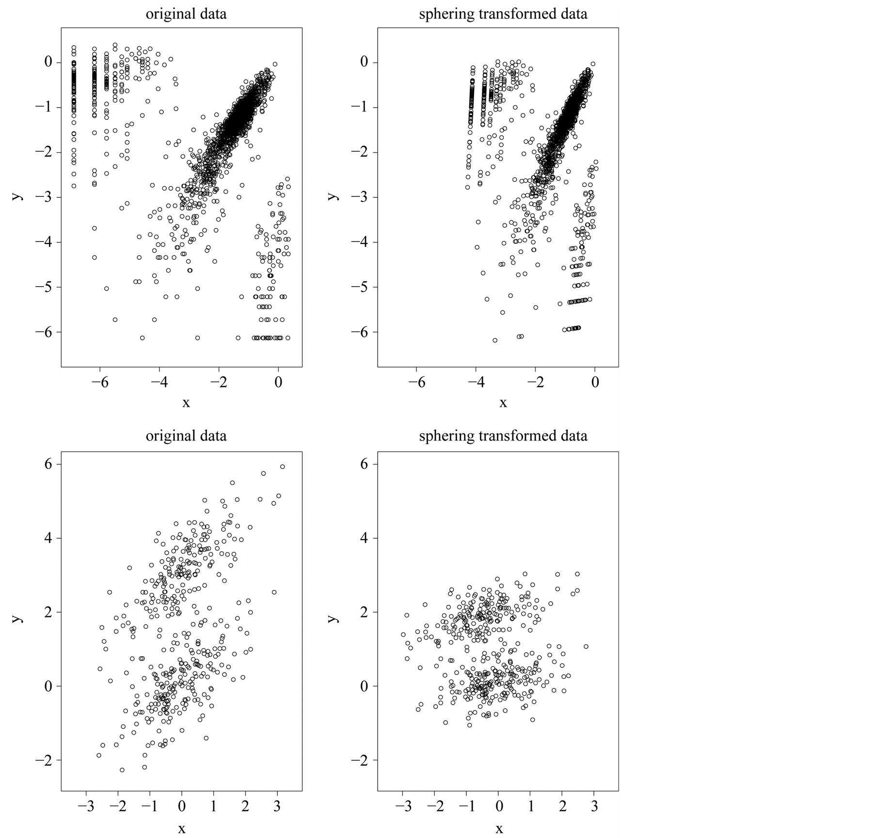
Figure 1. Two examples of original data and sphering transformed data.
and the minimized AMISE is:

The “normal reference rule” [11] is widely used. It is given as:

where
 is the standard deviation of the jth dimension and can be estimated by the corresponding sample standard deviation.
2.3. Asymptotic Distribution of KDE
In this section, we review the details of the asymptotic properties of KDE defined in (1.4).

As , we have

showing that
 is asymptotically unbiased. We apply the normal reference rule on the sphering transformed data to choose the bandwidth parameter h as (2.2),

Note that the term . If we choose h with the optimal convergent rate, which is
 defined as (2.2), for example, using normal reference rule, then

The kernel density estimator has the following asymptotic normality property of:
Property 1. If
 and
and
 as
as
 then
then
 .
.
The proof of the above property is based on the Liapunov Central Limit Theorem. [12] provide the details of the proof. From the Property 1, it can be seen that by choosing the
 at optimal convergent rate, the KDE
 asymptotically is a biased estimator of
 . It underestimates the local maxima since the term
 in bias is negative at maxima and it overestimates at local minima due to the same reason.
If we choose an h that converges faster than the optimal rate, i.e.,

the bias term can be made negligible. The asymptotic distribution then becomes:
Property 2. If ,
,
 and
and
 as
as , then
 .
.
To satisfy the conditions
 and
and , we should choose
 as
as

If the h converges slower than the optimal rate, the bias term cannot converge as .
.
Note that the variance term in the asymptotic distribution contains the unknown parameter . Simply by applying the delta method and using the transformation function
 , the variance is stabilized and becomes invariant with
 . The asymptotic distribution in Property 1 becomes

Further, it is easy to verify the following property:
Property 3. If
 and
and
 as
as , for
, for ,
,
 and
and
 are uncorrelated.
Proof: We consider the covariance between
 and
and .
.

We want to show that
 if
if
 and
and
 as
as . Consider the term

For the second last step, since
 is a convolution and hence another density, therefore its integration is bounded by 1. Now we consider the term

Thus, it follows

Therefore, we proved that
 and
and
 are asymptotically uncorrelated. Since under the same condition of Property 3,
 and
and
 asymptotically follow normal distributions, we can claim they are asymptotically independent.
3. Mode and Ridgeline
[1] proposed a set of comprehensive tools to explore the geometric feature of the KDE. In this section, we review the basic quantities of the modality inference, which are the mode, the saddle point and the ridgeline. We will also discuss the algorithms to determine these quantities under the KDE.
3.1. Mode
Mode is defined as the local maximum of a probability density. Traditional techniques of finding local maxima, such as hill climbing, work well for univariate data. However, multivariate hill climbing is computationally expensive, thereby limiting its use in high dimensions. [1] proposed an algorithm that solves a local maximum of a KDE by ascending iterations starting from the data points. Since the algorithm is very similar to the expectation maximization (EM) algorithm [13] , it is named as the modal expectation maximization (MEM). The finite mixture model can be expressed as
 (1.5)
(1.5)
with
 and
and
 are the mixing components. Given any initial value
 , the MEM solves the local maxima of the mixture density by alternating the following two steps until it meets some user defined stopping criterion.
Step 1: Let

Step 2:

Details of convergence of the MEM approach can be found in [1] . The above iterative steps provide a computationally simpler approach than the grid search method for hill climbing from any starting point , by exploiting the properties of density functions. Given a multivariate kernel K, let the density of the data be given by
 , where
 is the matrix of smoothing parameters. Moreover, in the special case of Gaussian kernels, i.e.,
 , where
 is the pdf of a Gaussian distribution, the update of
 is simply

This allows us to avoid the numerical optimization of Step 2. Due to this reason, the normal kernel function is used throughout the methods introduced in this thesis. However, in general, one can also use other kernel functions.
The MEM algorithm can be naturally used to define clusters. If we start the algorithm from each data point, we can cluster the data that converges to the same mode as one group. [1] denotes this algorithm the Mode Association Clustering (MAC). If we choose a sequence of bandwidth parameters h, then we can get the Hierarchical MAC (HMAC).
3.2. Saddle Point and Ridgeline
[14] provided the explicit formula for the ridgeline between the two means of the mixture of two multivariate normal distributions. The mixture density of two d-dimensional multivariate normal distributions is:
 (1.6)
(1.6)
where the
 and
and
 are the mean vectors and
 and
and
 are the two covariance matrices of the two mixed multivariate normal components respectively. The ridgeline of the distribution in (1.6) from one mean to another is given by:
 (1.7)
(1.7)
where
 and
and . [14] showed that all the critical points of the d-dimensional distribution, including the modes and saddle points, are the points on the ridgeline. With different choices of the parameters, the probability density can be unimodal, bimodal or in some special cases, trimodal. See some examples in [15] . The ridgeline provides a useful tool to discover the modality of a mixture of multivariate normal mixtures.
[1] also provided the algorithm to find the ridgeline of the KDE between the two modes identified by MEM, named the Ridgeline EM (REM). Here we provide a brief description of the REM:
Let the density of the two clusters represented by the two modes of interest be
 and
and . We can consider both
 and
and
 as the mixtures of
 parametric distributions:

Starting from an initial value , the REM updates x by iterating the following two steps:
Step 1: Compute:
 with
with

Step 2: Update :
:

In the special case where , the multivariate normal distribution, the second step becomes
 Figure 2 illustrates one example of the ridgeline.
The point on the ridgeline with the lowest density is the detected saddle point. The REM and MEM introduced in this section provide useful tools to detect the mode and saddle point of the KDE, which provides the basis of the inferential framework introduced in the following section.
4. Test Statistic and Its Asymptotic Distribution
We denote the one of
 and
and
 with lower density by
 . To test the hypothesis defined in (1.2), a natural choice is to compare the density of
 against the density of the saddle point
 , which is the point on the ridgeline between
 and
and
 with minimum density. We use Ridgeline EM (REM), which was reviewed in Section 1.3 to determine the saddle point
 . To identify the interested pair of modes, in practice, when several modes are identified by MEM, it starts with the one with the lowest density and its neighbor mode. Or, one can select the particular pair of modes based on the context of the study. After identifying
 and
and , the hypothesis in (1.2) can be restructured as:
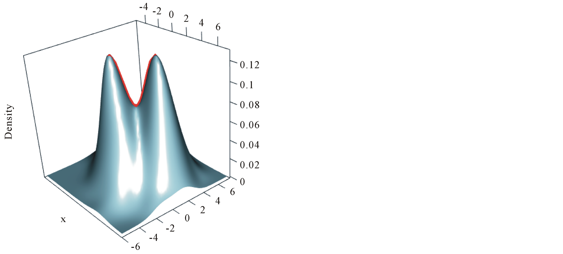
Figure 2. Ridgeline example.
 (1.8)
(1.8)
We use
 and
and
 to make the inference, where
 is the kernel density estimate of
 and
and
 and
and
 are the estimated mode and saddle point of the KDE detected by the Modal EM (MEM) algorithm, which was reviewed in Section 3. We believe
 is a good estimation of the modal region and is close to the true population mode, and same for the
 .
.
Theorem 1. Using Gaussian kernel function, under
 of (1.8), if
 ,
,
 and
and
 as
as , then
 (1.9)
(1.9)
Proof: Using Property 2, Property 3 and density in 1.5, we can show that:
 (1.10)
 and
and
 are correlated. However, based on Property 3, as long as
 ,
,
 and
and
 are asymptotically independent.
Next, we simplify the term . For univariate standard normal kernel function:
 , we have
 . Therefore, for d-dimensional multivariate normal kernel function:
 , we have
 . Thus we prove the theorem. This is the test statistic of Hypothesis (1.8) and its asymptotic distribution.
5. Choice of the Bandwidth Parameter
In order to use the asymptotic distribution (1.9), the conditions of Property 2 must be satisfied. To satisfy the conditions
 and
and , the bandwidth parameter
 should be chosen as

However, the range of ,
,
 , is still wide if the dimension of the data is not high, e.g.,

if . Theoretically, the bias of the KDE can be negligible if
 is within this interval. However, in practice, the selection of
 affects the variance-bias trade off, which affects the inference dramatically. We demonstrate the phenomenon using logctA20 data set. The description of the data set can be found in R package Modalclust, which will be described in the next chapter. logctA20 is a two-dimensional data with 2166 observations. The scatter plot of the data is shown in Figure 3.
Using the normal reference rule, the bandwidth parameter used for the MEM is:

Using the MAC to cluster the data, the output shows that there are four major clusters. Figure 4 shows the clustering output as well as the modes, saddle points and ridgeline between the modes. The next step is to test if
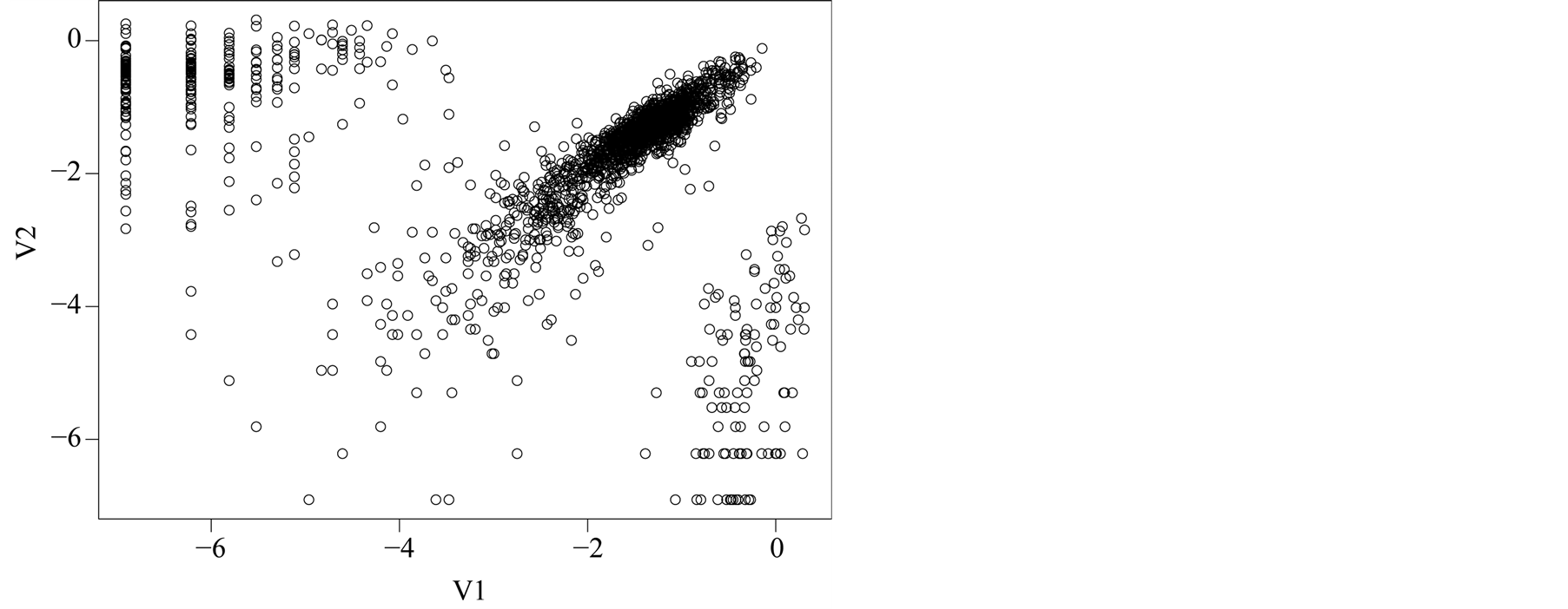
Figure 3. Scatter plot of logctA20 data.
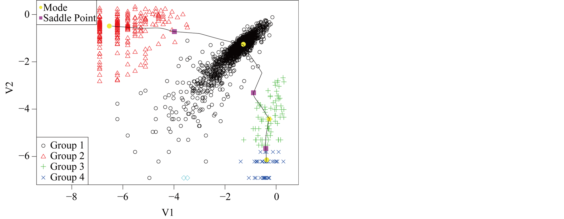
Figure 4. Mode, saddle point and ridgeline of logctA20 data.
the four modes are significant. We consider three tests for the three adjacent pairs of modes: the test of Mode 4 against Mode 3, Mode 3 against Mode 1 and Mode 2 against Mode 1. As mentioned at the beginning of this section, in order to use the asymptotic distribution (1.9), we should choose the bandwidth parameter h so that it converges faster than the optimal rate. Thus, we should choose

Figure 5 provides the plot of the p-value of the modality test against the choice of the . It clearly demonstrates that the value of the
 affects the conclusion of the inference. For Mode 2, the lower values of
 lead to rejecting the null hypothesis, whereas the higher values of
 lead to not rejecting the null hypothesis, In practice, if we choose a small value of
 , the bias term still exists, even though asymptotically it will converge to 0. If we choose a large value of
 , the variance is relatively large and could mislead the conclusion. We suggest to use a small value of
 , which will lead to a large value of
 .
.
Remark: Recall in Section 2, we reviewed that the bias term in Property 1 is .
.
Note that
 at
at
 and
and
 at
at . Thus, under
 of hypothesis in (1.8), the expectation of the test statistic is negative if the bias exists. Therefore, it makes the test conservative.
From the analysis in Figure 5, we conclude that Mode 4 is not significant, while Mode 2 and Mode 3 are.
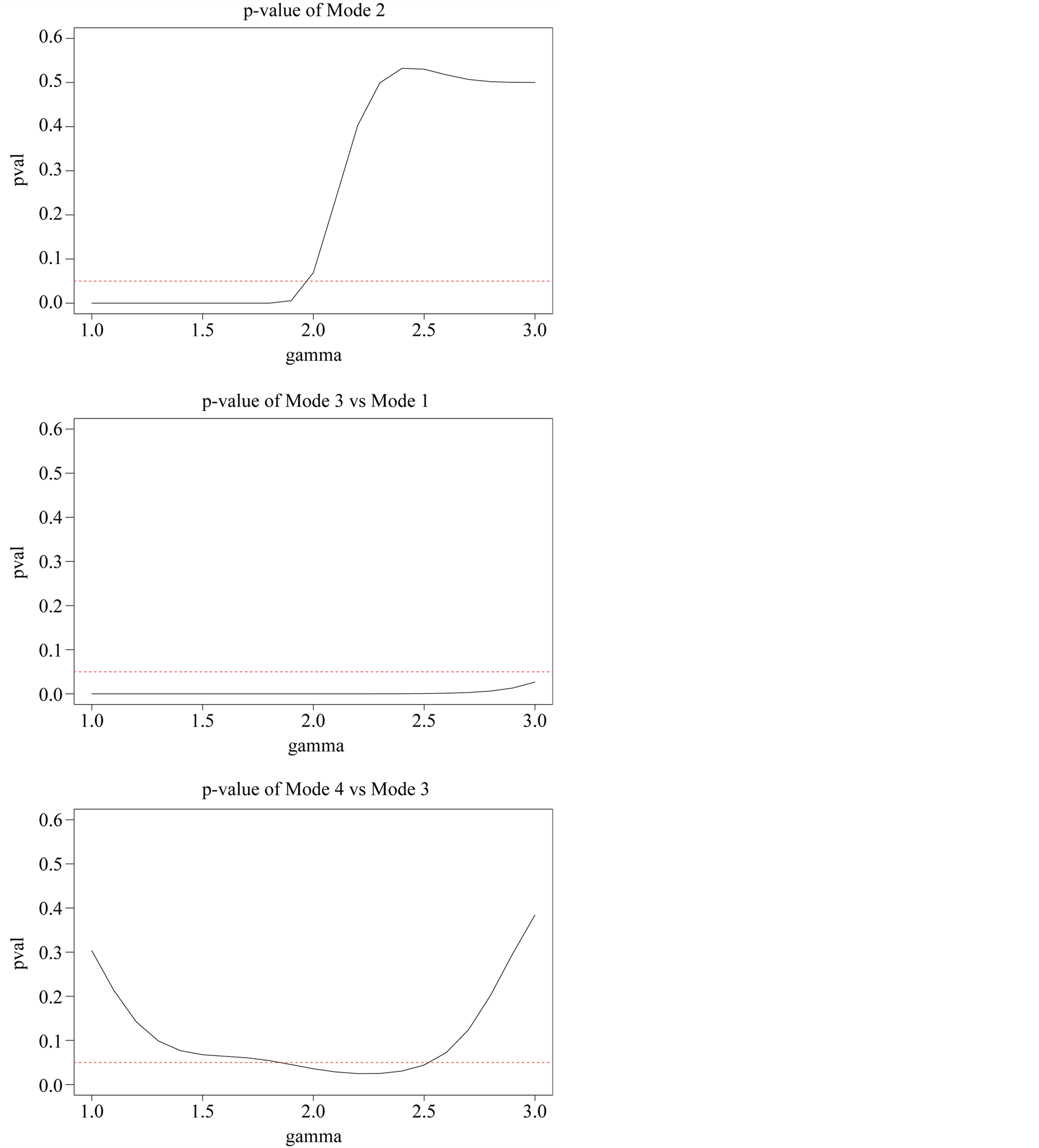
Figure 5. p-value of modality inference against γ.
Group 4 can be merged with Group 3. The final plot after merging Group 4 with Group 3 is given in Figure 6. Note that the resulting modes are all significant.
When we have several mode candidates and when we want to inference on the entire distribution to see how many significant modes, there is a multiplicity issue. One can refer [15] for some method to control the overall Type I error rate. We focus on the local significance and do not provide an overall significance of the final result.
6. The Procedure of the Mode Hunting and Inference
The inference procedure proposed in the previous section, along with the MEM and REM reviewed in Section 3, provides a comprehensive tool for mode hunting and follow-up inference of a data set. In this section, we summarize the procedure.
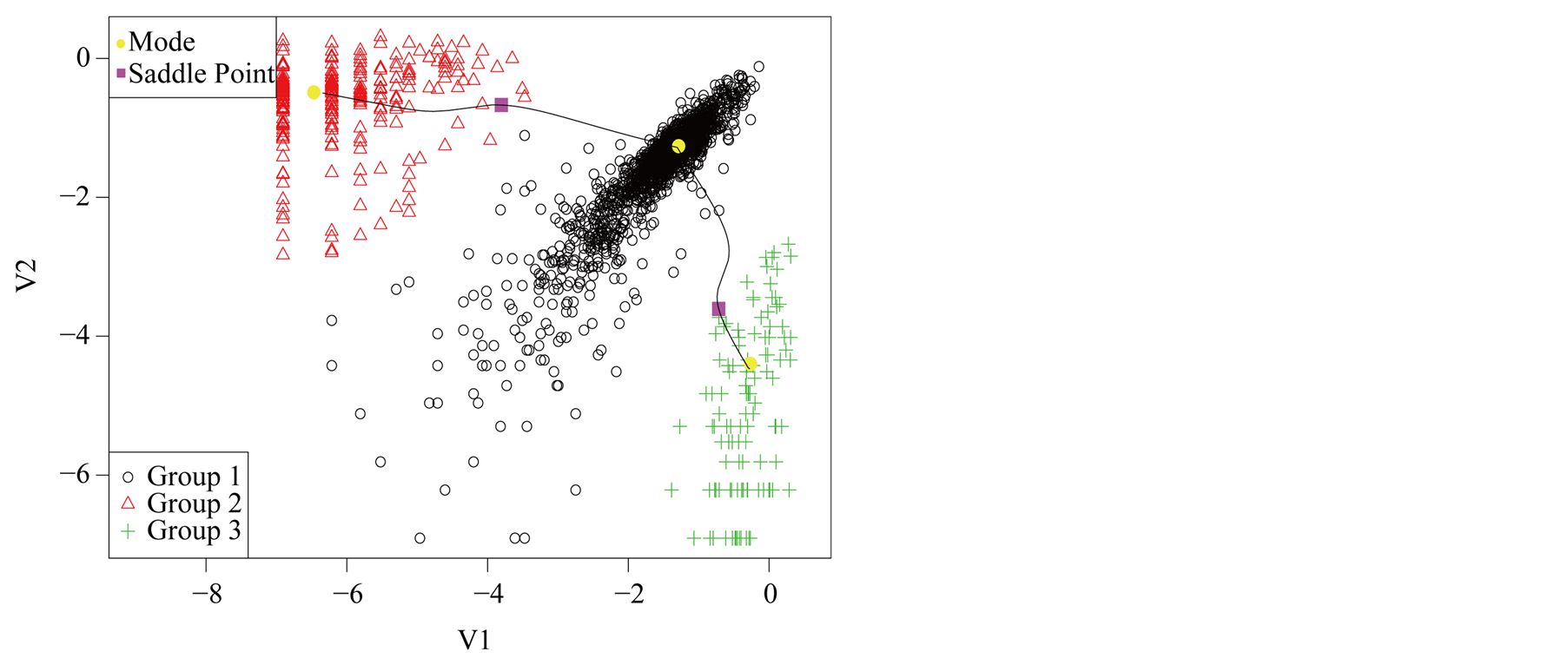
Figure 6. Mode, saddle point and ridgeline of the example data after merging.
Step 1: Sphering transformed the data;
Step 2: Use KDE to estimate the density of the data with bandwidth parameter chosen by some standard method, e.g., the normal reference rule, etc.;
Step 3: Identify the modes of KDE using MEM. After determining the pair of modes
 and
and , identify the corresponding saddle point
 by REM;
Step 4: Use
 where
where
 and
and
 to calculate
 and
and . In particular, we suggest to choose
 when d is small;
Step 5: Make the inference of the Hypothesis (1.8) based on the asymptotic distribution (1.9).
7. Application
This section provides the application of the modality inferential framework on some real and simulated data sets. We start by providing a description of the data sets and follow up by providing the conclusion of the inferential framework.
7.1. Four Discs
The four disks data is a simulated data. It contains 10,000 observations and the data is a mixture of four bivariate normal distributions. The mean vectors are ,
,
 ,
,
 ,
, .
.
The data contains multiple layers of the clusters. There are three main clusters with one of them having two sub-clusters. By the simulation design, the Group 1 and 2 shown in Figure 7 are two distinct groups. The p-value of Mode 1 compared with Mode 2 is 0.0194. However, Group 1 and 2 are relatively close compared to the other groups. After merging these two groups together, the resulting clusters and the ridgeline between each pair of modes are shown in Figure 8. The multiple layers of clusters are common in real life application. The decision of how many clusters the data has is often related to the application area and research question.
7.2. 3-Dimensional Two Half Discs
The 3-dimensional two half discs is another simulated data set with 800 samples. It is formed by two half discs with equal size, i.e. 400 samples for each disc. Using
 and
and
 for
for

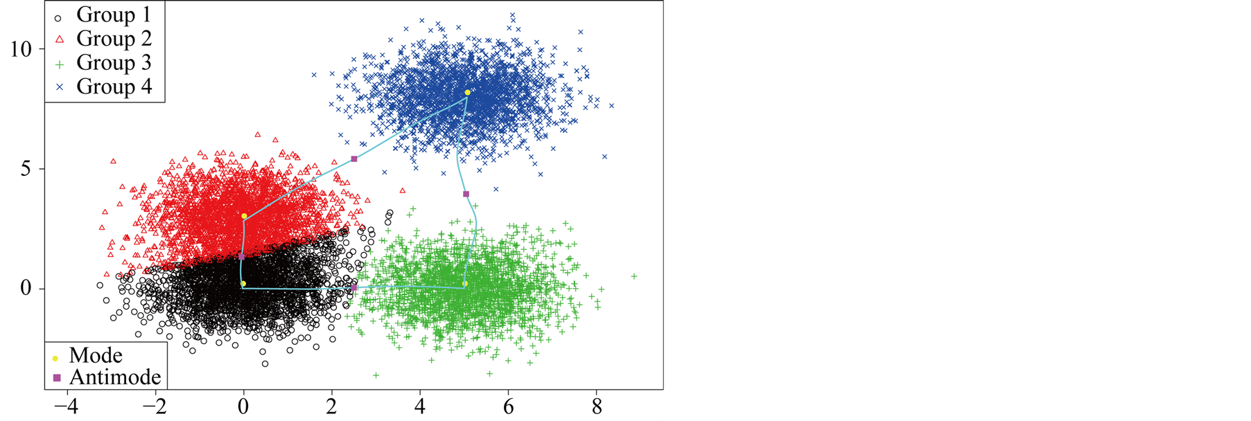
Figure 7. The first layer of four discs data.
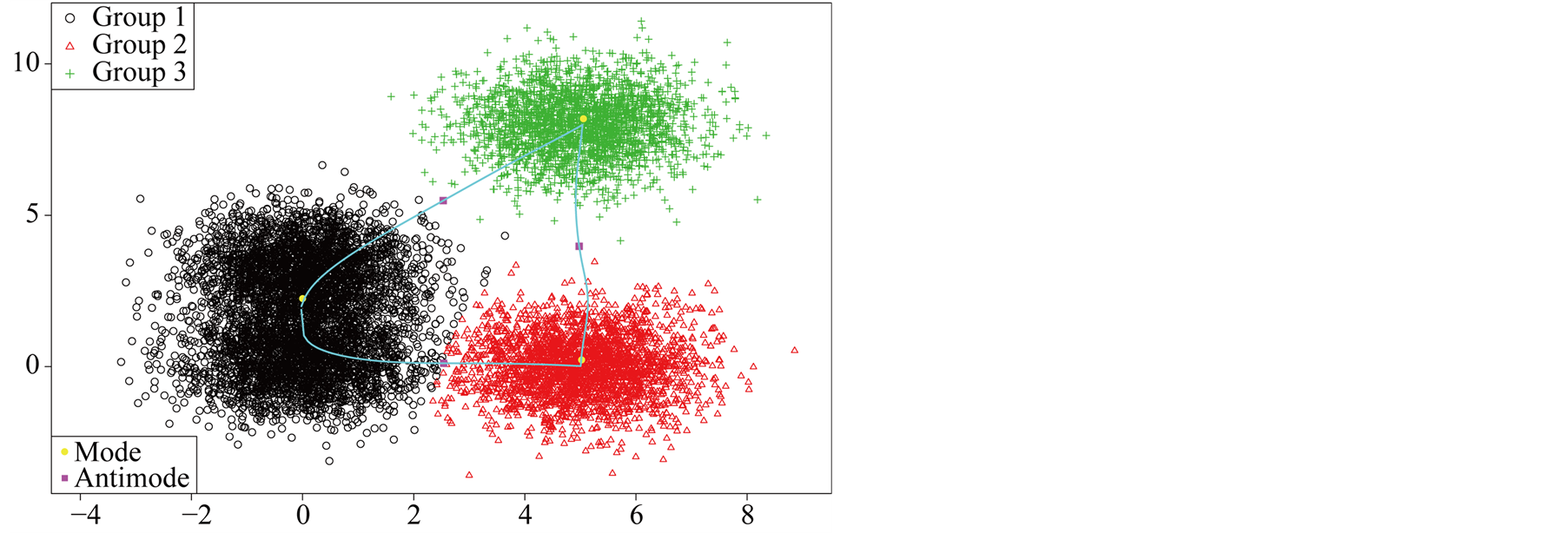
Figure 8. The second layer of four discs data.
we get . The clustering output using the MAC with
 is shown in Figure 9. There are 4 major clusters and the number of samples of each cluster is given in Table1
The inference between some major clusters is carried out and the resulting p-values are given in Table2 It is straightforward to conclude that Group 1 is not significantly distinct from Group 3, and Group 6 is not distinct from Group 5. Group 3 is significantly separated from Group 5 and 6. Group 5 is significantly separated from Group 1 and 3. Thus, we get the conclusion that there are two main groups in this data set.
7.3. Flow Cytometry Data
Flow cytometry is a technology that simultaneously measures and then analyzes multiple physical characteristics of single cell, as they flow in a fluid stream through a beam of light. Flow cytometry is one of the most commonly used platforms in clinical and research labs worldwide. It is used to identify and characterize types and functions of cell populations e.g., dead or live cells, in a sample by measuring the expression of specific proteins on the surface and within each cell.
Flow cytometry data consists of per cell measurements (or events) in the form of scattering of light and fluorescence intensity from the fluorophore-conjugated markers. In a typical flow data analysis workflow, a human analyst visually inspects 2-dimensional scatter plots of a sample, where the dimensions could be scatters, marker intensities, or a combination of these, and it demarcates (or gates) specific populations of interest such as live cells, lymphocytes, etc. Often, gates are drawn around visually discernible congregations of events. For instance, for live gating, the dead cells or debris could be discerned by their small cell size and granularity, which appear as a distribution of points with low forwardand side-scatter values. Forward-scatter light (FSC) and Side-scatter light (SSC) reflects two features of the cells and forms a two-dimensional scatter plot. FSC is proportional to cell-surface area or size. SSC is proportional to cell granularity or internal complexity. The manual approach to gating is, however, labor-intensive and subjective, and gating results can vary considerably from one analyst

Figure 9. 3-D two half discs data.

Table 1. Cluster size of two half discs data.
Table 2. p-value of modality inference on two half discs data.
to another. [16] have used the MAC to gate flow cytometry data. However, the inference is distinctly missing. Figure 10 is one example of flow cytometry data. The data contains 4905 cells. In this plot, the dead cells have a relatively smaller size compared with the live cells, which shows that the dead cells have a smaller value of FSC and SSC. In the scatter plot, the dead cells are at the bottom left corner. For this data set, using the inference procedure introduced in Section 6, we applied the MAC on the data with
 and got the two major clusters. It is suspected that the cluster on the bottom left represents the dead cells, while the rest are the live cells. The p-value of the mode existence inference is
 . Thus, the procedure can automatically identify the dead cell population distinctly from the live cells.
7.4. Swiss Banknotes
The data set contains 6 measures of 200 Swiss banknotes, where 100 are real and 100 are counterfeit. The 6 measures are:
 : Length of the bank note,
 : Height of the bank note, measured on the left,
 : Height of the bank note, measured on the right,
 : Distance of inner frame to the lower border,
 : Distance of inner frame to the upper border,
 : Length of the diagonal of the inner image.
All measurements are in millimeters. The original banknote image and the measurements are shown in Figure 11. In this data set, we know the truth of whether the banknote is real or forged. More information about the data set can be found in [17] . We use the spectral degrees of freedom concept, which was proposed by [18] , and supply
 for the MAC. The MAC output shows there are two major clusters and can capture the two groups well. The output is shown in Table3 Group 1 and Group 4 are the two major clusters. Using
 , the p-value of the corresponding modality inference is 0.001774, which indicates the two clusters are clearly separated.
8. Discussion
In this paper, we developed the inference procedure to test the significance of a specific mode. The asymptotic distribution of the test statistic is derived based on the asymptotic normality of the KDE to assess the significance of the mode. The traditional method to assess the significance of the modality of the data is to determine the test statistic and decide the reference distribution under the null hypothesis. Then, a large scale simulation is performed to simulate the reference data and compute the test statistic of the simulated reference data to form
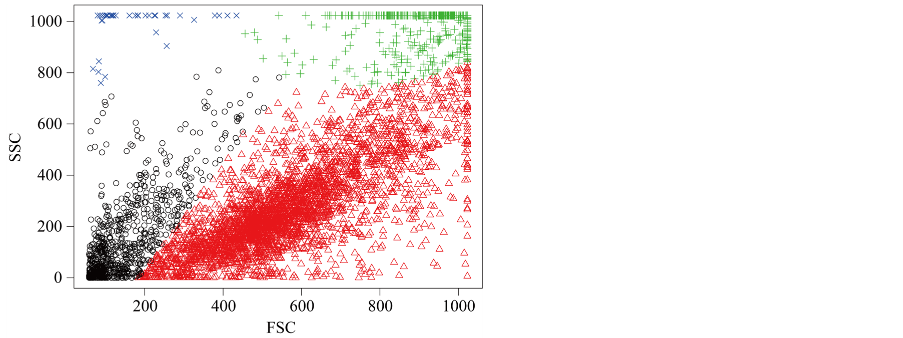
Figure 10. One example of flow cytometry data clustered by MAC.
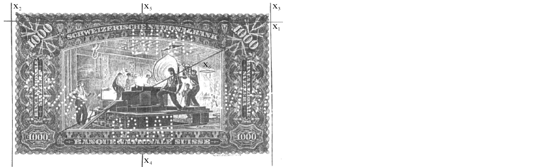
Figure 11. 6 measurements of Swiss banknote data.
Table 3. MAC output of emphSwiss banknotes data.
the null distribution of the test statistic. The method we introduced uses the asymptotic distribution of the statistic, thus, we can avoid the bootstrap testing, which could be computationally expensive.
Combined with the research work in [1] , we provided a comprehensive mode hunting and inference tool for the investigated data set. The mode hunting and inference procedure is based on the KDE and using the normal density as the kernel function. It is important to select the bandwidth parameter h. There are two steps to select the bandwidth parameters. It is acknowledged that there is no best choice of h for estimating a density. For mode hunting, we chose to use the normal reference rule. For the inference, h has to satisfy the conditions of the asymptotic normality of the KDE. Due to the curse of the dimensionality, this method is limited to low or moderate dimensions.
We can apply this inference procedure on each pair of modes to assess how many modes the data have. In the MAC algorithm, the number of modes is the same as the number of clusters. It is difficult but worthwhile to generate the automated algorithm to decide on how many clusters/modes of the data have, based on the modality inference procedure. The difficulty here is that the method is based on the KDE. The outliers of the data could easily form the spurious modes, especially for the high dimensional data, which make it difficult to generate automated algorithm.
References
- Li, J., Ray, S. and Lindsay, B.G. (2007) A Nonparametric Statistical Approach to Clustering via Mode Identification. Journal of Machine Learning Research, 8, 1687-1723.
- Tibshirani, R., Walther, G. and Hastie, T. (2001) Estimating the Number of Clusters in a Data Set via the Gap Statistic. Journal of the Royal Statistical Society: Series B (Statistical Methodology), 63, 411-423.http://dx.doi.org/10.1111/1467-9868.00293
- McLachlan, G. and Peel, D. (2004) Finite Mixture Models. Wiley, Hoboken.
- Lloyd, S. (1982) Least Squares Quantization in PCM. IEEE Transactions on Information Theory, 28, 129-137. http://dx.doi.org/10.1109/TIT.1982.1056489
- Fraley, C. and Raftery, A.E. (2002) Model-Based Clustering, Discriminant Analysis, and Density Estimation. Journal of the American Statistical Association, 97, 611-631. http://dx.doi.org/10.1198/016214502760047131
- Silverman, B.W. (1981) Using Kernel Density Estimates to Investigate Multimodality. Journal of the Royal Statistical Society, Series B (Methodological), 43, 97-99.
- Efron, B. (1979) Bootstrap Methods: Another Look at the Jackknife. The Annals of Statistics, 7, 1-26.http://dx.doi.org/10.1214/aos/1176344552
- Minnotte, M.C. (1997) Nonparametric Testing of the Existence of Modes. The Annals of Statistics, 25, 1646-1660.http://dx.doi.org/10.1214/aos/1031594735
- Burman, P. and Polonik, W. (2009) Multivariate Mode Hunting: Data Analytic Tools with Measures of Significance. Journal of Multivariate Analysis, 100, 1198-1218. http://dx.doi.org/10.1016/j.jmva.2008.10.015
- Fukunaga, K. (1990) Introduction to Statistical Pattern Recognition. Academic Press, Waltham.
- Scott, D.W. (1992) Multivariate Density Estimation: Theory, Practice, and Visualization. John Wiley, New York.
- Li, Q. and Racine, J.S. (2011) Nonparametric Econometrics: Theory and Practice. Princeton University Press, Princeton.
- Dempster, A.P., Laird, N.M. and Rubin, D.B. (1977) Maximum Likelihood from Incomplete Data via the EM Algorithm. Journal of the Royal Statistical Society, Series B (Methodological), 39, 1-38.
- Ray, S. and Lindsay, B.G. (2005) The Topography of Multivariate Normal Mixtures. The Annals of Statistics, 33, 2042-2065. http://dx.doi.org/10.1214/009053605000000417
- Dmitrienko, A., Tamhane, A.C. and Bretz, F. (2010) Multiple Testing Problems in Pharmaceutical Statistics. CRC Press, Boca Raton.
- Ray, S. and Pyne, S. (2012) A Computational Framework to Emulate the Human Perspective in Flow Cytometric Data Analysis. PloS One, 7, Article ID: e35693. http://dx.doi.org/10.1371/journal.pone.0035693
- Flury, B. and Riedwyl, H. (1988) Multivariate Statistics: A Practical Approach. Chapman & Hall, Ltd., London. http://dx.doi.org/10.1007/978-94-009-1217-5
- Lindsay, B.G., Markatou, M., Ray, S., Yang, K. and Chen, S.C. (2008) Quadratic Distances on Probabilities: A Unified Foundation. The Annals of Statistics, 36, 983-1006. http://dx.doi.org/10.1214/009053607000000956