ABSTRACT

This article introduces a resampling procedure called the truncated geometric bootstrap method for stationary time series process. This procedure is based on resampling blocks of random length, where the length of each blocks has a truncated geometric distribution and capable of determining the probability p and number of block b. Special attention is given to problems with dependent data, and application with real data was carried out. Autoregressive model was fitted and the choice of order determined by Akaike Information Criterion (AIC) and Bayesian Information Criterion (BIC). The normality test was carried out on the residual variance of the fitted model using Jargue-Bera statistics, and the best model was determined based on root mean square error of the forecasting values. The bootstrap method gives a better and a reliable model for predictive purposes. All the models for the different block sizes are good. They preserve and maintain stationary data structure of the process and are reliable for predictive purposes, confirming the efficiency of the proposed method.

1. Introduction

The heart of the bootstrap is not simply computer simulation, and bootstrapping is not perfectly synonymous with Monte Carlo. Bootstrap method relies on using an original sample or some part of it, such as residuals as an artificial population from which to randomly resampled [1]. Bootstrap resampling methods have emerged as powerful tools for constructing inferential procedures in modern statistical data analysis. The Bootstrap approach, as initiated by [2], avoids having to derive formulas via different analytical arguments by taking advantage of fast computers. The bootstrap methods have and will continue to have a profound influence throughout science, as the availability of fast, inexpensive computing has enhanced our abilities to make valid statistical inferences about the world without the need for using unrealistic or unverifiable assumptions [3].

An excellent introduction to the bootstrap maybe found in the work of [4-9]. Recently, [10,11] have independently introduced non-parametric versions of the bootstrap that are applicable to weakly dependent stationary observations. Their sampling procedure have been generalized by [12,13] and by [14] by resampling “blocks of blocks” of observations to the stationary time series process.

In this article, we introduce a new resampling method as an improvement on the stationary bootstrap of [15] and the moving block bootstrap of [16,17].

The stationary bootstrap is essentially a weighted average of the moving blocks bootstrap distributions or estimates of standard error, where the weights are determined by a geometric distribution. The difficult aspect of applying these methods is how to choose b in moving blocks scheme and how to choose p in the stationary scheme.

On this note we propose a stationary bootstrap method generated by resampling blocks of random size, where the length of each block has a “truncated geometric distribution”.

In Section 2, the actual construction of a truncated geometric bootstrap method is presented. Some theoretical properties of the method are investigated in Section 3 in the case of the mean. In Section 4, it is shown how the theory may be extended to stationary time series processes.

2. Material and Method

To overcome the difficulties of moving blocks and geometric stationary scheme in determining both b (number of blocks) and p (probabilities). We introduced a truncated form for the geometric distribution and then demonstrated that it is a suitable model for a probability problem. This truncation is of more than just theoretical interest as a number of application has been reported [18,19].

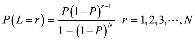
A random length L may be defined to have a truncated geometric distribution with parameter P and N terms, when it has the probability distribution or probability density function

(2.1)

The constant K is found, using the condition

, to be

Thus, we have

(2.2)

These are the probabilities of a truncated geometric distribution with parameter P and N terms. Suppose that L length, number 1 to N are to be selected randomly with replacement. Then, the process continues until it is truncated geometrically at r with an appropriate probability P attached to its random selection in form of,. We take our N to be 4, that is, the random selections could be truncated between 1 to 4 at an appropriate probabilities.

Then, a description of the resampling algorithm when r > 1 is as follows:

1) Let   be a random variables.

2) Let be determined by the r-th truncated observation X_r in the original time series.

3) Let be equal to X_r+1 with probability 1 – P and picked at random from the original N observations with probability p.

4) Let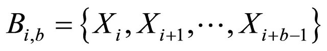, be the block consisting of b observation starting from X_i.

5) Let 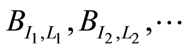be a sequence of blocks of random length determined by truncated geometric distribution.

6) The first L₁, observations in the pseudo time series are determined by the first block_, of observation the next L₂ observations in the pseudo time series are the observations in the second sampled block_.

7) The process is resampled with replacement, until the process is stopped once N observation in the pseudo time series have been generated.

8) Once has been generated, one can compute the quantities of interest for the pseudo time series.

The algorithm has two major components, the construction of a bootstrap sample and the computation of statistics on this bootstrap sample, and repeat these operation many times through some kinds of a loop.

Proposition 1. Conditional on, is stationary.

If the original observations are all distinct, then the new series is, conditional on, a stationary Markov chain. If, on the other hand, two of the original observations are identical and the remaining are distinct, then the new series is a stationary second order Markov chain. The stationary bootstrap resampling scheme proposed here is distinct from the proposed by [20] but posses the same properties with that proposed by [21].

3. Result and Discussion

In this section, the emphasis is on the construction of valid inferential procedures for stationary time series data, and some illustrations with real data are given. The real data are the geological data from demonstratigraphic data from Batan well at 30 m regular interval, [22]. The data is the principal oxide of sand or sandstone, which is S_iO₂ or silicon oxide. The point is that the bulk of oil reservoir rocks in Nigeria sedimentary basins is sandstone and shale, a product of sill stone [23]. In other to improve on the geological analysis and prediction of the presence of these elements, a mathematical tool which can be used to examine a wide range of data sets is developed to detect and improve new and old oil basins.

The geological data of 130 observations was subjected to our new method described in section two of this article at 500 and 1000 bootstrap replicates, for block of (1, 2, 3, and 4).

The replicates with minimum variance was selected in each case of number of bootstrap replicates.

3.1. Model Fitting, Normality Test and Forecasting

The linear models are fitted and consider the choice of the order of the linear model on the basis of Akaike Information Criterion (AIC), Bayesian Information Criterion (BIC) and residual variance_, [24].

Fitting of AR Models to Bootstrapped Data

The linear models were fitted to the bootstrapped observations when the bootstrap replicates are (B = 500, B = 1000) for blocks of (1, 2, 3 and 4). When B = 500 replicates, we have the following models.

wang#title3_4:spBlock 1:

It is found that AIC and BIC is minzimum at P = 4.

The fitted model is

(3.1)

Block 2:

The fitted model is:

(3.2)

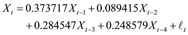
wang#title3_4:spBlock 3:

The model fitted is:

(3.3)

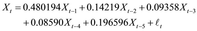
wang#title3_4:spBlock 4:

The fitted model is:

(3.4)

The table below shows the value of, AIC and BIC for blocks (sizes) when B = 500 replicates.

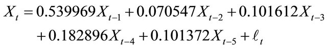
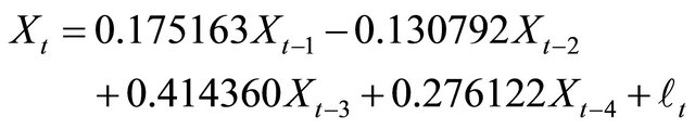
When B = 1000 replicates

wang#title3_4:spBlock 1:

The fitted model is:

(3.5)

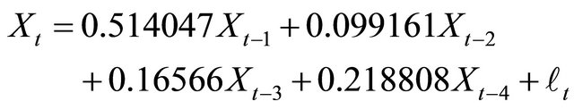
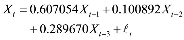
Block 2:

(3.6)

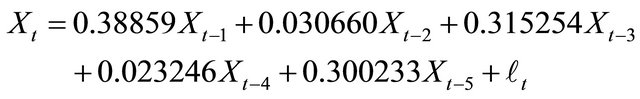
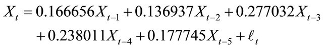
wang#title3_4:spBlock 3:

The fitted model is:

(3.7)

wang#title3_4:spBlock 4:

The fitted model is:

(3.8)

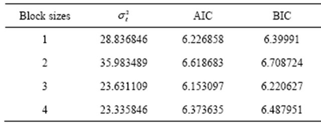
The table below summarizes the value of, AIC and BIC for blocks (sizes) when B = 1000 replicates.

From Tables 1 and 2, it observed that the residual variance for each block sizes are moderate, indicating a selection procedure from any of the models retain the time series data structure and any prediction from it is reliable.

3.2. Normality Test for Residual of Fitted Models

An important assumption we have made in fitting the linear and non-linear models to data is that the error of the model are mutually independent and normal. If a model is fitted to some data it may be appropriate to see whether the assumption is satisfied. Once it is satisfied

Table 1. Measure of goodness fit by block sizes for 500 replicates.

Table 2. Measures of goodness of fit by block sizes for 1000 replicates.

one can consider the model suitable for forecasting.

The normality test for residuals of fitted models is carried out using Jargue-Bera statistic tests (JB). At 5% level of significance with 2 degree of freedom the critical values of is 5.99, (15) So, if JB > 5.99, one rejects the null hypothesis that the test is normal.

Test for AR models of 500 replicates

H₀: The test is normal H₁: The test is not normal

Table 3 reveals that the test is normal in all the block sizes.

Test for AR models of 1000 replicates

H₀: The test is normal H₁: The test is not normal

Table 4 reveals that the test is normal in all block sizes.

Therefore, the normality test carried out in this article reveals that the proposed truncated geometric bootstrap method for dependent data at different replications is normal in all block sizes and any forecast from this models are good. That is, the residual of the models satisfied the normality test.

3.3. Forecasting

The linear models are fitted and then prediction or forecast are calculated for the next 10 observations. The following are the forecast values for 500 and 1000 replicates of different block sizes.

The forecast values for the replication of different block sizes from the Tables 5 and 6 reveals that while the probability forecast increases that of elementary forecast are not stable over time. The forecast shows a decline values throughout the period, except for block of

Table 3. Summary for JB statistics, B = 500.

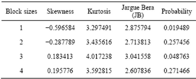
Table 4. Summary for JB statistics, B = 1000.

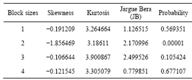
Table 5. Forecast values for B = 500 replicates.

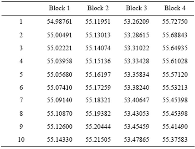
Table 6. Forecast values for B = 1000 replicates.

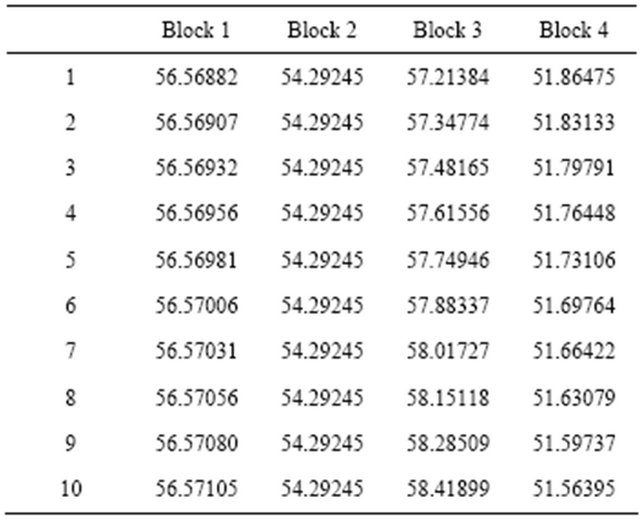
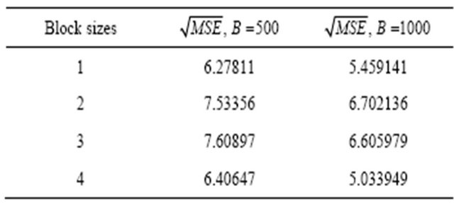
Table 7. Root mean square error, for the forecast value.

3, that shows upward values throughout the period.

In order to justify the best model for prediction, one must consider the root mean square error of the forecast values. Table 7 is some of root mean square error of the forecast values.

To measure and establish the best model, we use the root mean square error of the forecast values. The above table reveals that the values are moderate for all the models in all bootstrap replicates. Therefore models fitted for all block of sample sizes are the best model for prediction purposes.

4. Summary and Conclusions

The truncated geometric bootstrap method proposed in this article is able to determine P in (0, 1) and provides b, for stationary time series process.

We proposed an algorithm for effective truncated geometric bootstrap method, which shares the construction of resampling blocks of different sizes of observation to form pseudo-time series, so that the statistics of interest are calculated along based on the resampled data sets. We implemented this method with real geological data and generated bootstrap replications of (B = 500 and 1000) for different block sizes of (b = 1, 2, 3, 4) which represents each number of truncations.

The linear models of AR (10) are fitted to the resampled pseudo-time series data, and the choice of the order are determined by AIC and BIC. The normality test was carried out using Jargue Bera statistic on the residual variance of the fitted models. Forecast was generated for the next 10 observations based on the fitted models, which are justified by root mean square error of the models.

In conclusion, the bootstrap method gives a better and a reliable models for predictive purposes. All the models for the different block sizes are good. They preserve and maintain stationary data structure of the process and are reliable for predictive purposes, confirming the efficiency of the proposed method.

REFERENCES

- G. A. Bancroft, D. J. Colwell and J. R. Gillet, “A Truncated Poisson Distribution,” The Mathematical Gazette, Vol. 67, No. 441, 1983, pp. 216-218. doi:10.2307/3617187
- H. Barreto and F. M. Howland, “Introductory Econometrics, Using Monte Carlo Simulation with Microsoft Excel,” Cambridge University Press, Cambridge, 2005. doi:10.1017/CBO9780511809231
- D. Brillinger, “Time Series: Data Analysis and Theory,” Holen-Day, San Francisco, 1981.
- A. C. Davison and D. V. Hinkley, “Bootstrap Methods and Their Application,” Cambridge University Press, Cambridge, 1997.
- T. Diciccio and J. Romano, “A Review of Bootstrap Confidence Intervals (with Discussion),” Journal of the Royal Statistical Society, Vol. 50, 1988, pp. 338-370.
- B. Efron, “Bootstrap Methods Another Look at the Jacknife,” Annals of Statistics, Vol. 7, No. 1, 1979, pp. 1-26. doi:10.1214/aos/1176344552
- B. Efron and R. Tibshirani, “Bootstrap Measures for Standard Errors, Confidence Intervals, and Other Measures of Statistical Accuracy,” Statistical Science, Vol. 1, No. 1, 1986, pp. 54-77. doi:10.1214/ss/1177013815
- B. Efron and R. Tibshirani, “An Introduction to the Bootstrap,” Chapman and Hall/CRC, London, 1993.
- D. Hinkley, “Bootstrap Method,” Journal of the Royal Statistical Society, Vol. 50, 1988, pp. 321-337.
- C. H. Kapadi and R. L. Thomasson, “On Estimating the Parameter of the Truncated Geometric Distribution by the Method of Moments,” Annals of the Institute of Statistical Mathematics, Vol. 20, 1975, pp. 519-532.
- H. R. Kunsch, “The Jacknife and the Bootstrap for General Stationary Observations,” The Annals of Statistics, Vol. 17, No. 3, 1989, pp. 1217-1241. doi:10.1214/aos/1176347265
- C. Leger, D. Politis and J. Romano, “Bootstrap Technology and Applications,” Technometrics, Vol. 34, No. 4, 1992, pp. 378-398. doi:10.1080/00401706.1992.10484950
- R. Y. Liu and K. Singh, “Moving Blocks Jackknife and Bootstrap Capture Weak Dependence,” In: R. Lepage and L. Billard, Eds., Exploring the Limits of Bootstrap, John Wiley, New York, 1992.
- J. I. Nwackukwu, “Organic Matter, the Source of Our Wealth,” An Inaugural Lecture Delivered at Oduduwa Hall, Obafemi Awolowo, University of Ile-Ife, Ile-Ife, 2007.
- J. F. Ojo, T. O. Olatayo and O. O. Alabi, “Forecasting in Subsets, Autoregressive Models and Autoprojective Modes,” Asian Journal of Scientific Research, Vol. 1, No. 5, 2008, pp. 1-11.
- V. O. Olanrewaju, “Rocks: Their Beauty, Language and Roles as Resources of Economic Development,” An Inaugural Lecture Delivered at Oduduwa Hall, Obafemi Awolowo University, Ile-Ife, 2007.
- D. Politis and J. Romano, “A General Resampling Scheme for Triangular Arrays of a-Mixing Random Variables with Applications to the Problem of Spectral Density Estimation,” The Annals of Statistics, Vol. 20, No. 4, 1992, pp. 1985-2007. doi:10.1214/aos/1176348899
- D. Politis and J. Romano, “A Nonparametric Resampling Procedure for Multivariate Confidence Regions in Time Series Analysis, in Computing Science and Statistics,” In: C. Page and R. Lepage, Eds., Proceedings of the 22nd Symposium on the Interface, Springer-Verlag, New York, 1992, pp. 98-103.
- D. Politis and J. Romano, “The Stationary Bootstrap,” Journal of American Statistical Association, Vol. 89, No. 428, 1994, pp. 1303-1313.
- D. Politis, J. Romano and T. Lai, “Bootstrap Confidence Bands or Spectra and Cross-Spectra,” IEEE Transactions on Signal Processing, Vol. 40, No. 5, 1992, pp. 1206- 1215. doi:10.1109/78.134482
- M. B. Priestley, “Spectral Analysis and Time Series,” Academic Press, New York, 1981.
- M. Rosenblatt, “Asymptotic Normality, Strong Mixing and Spectral Density Estimates,” Annals of Probability, Vol. 12, No. 4, 1984, pp. 1167-1180.
- K. T. Sofowora, “Factor Analysis: Application with a Chemostratigraphic Data,” Department of Mathematics, Faculty of Science, Obafemi Awolowo University, Ile-Ife, 2002.
- I. G. Zurbenko, “The Spectral Analysis of Time Series,” North-Holland, Amsterdam, 1986.