Journal of Water Resource and Protection
Vol. 3 No. 2 (2011) , Article ID: 4051 , 13 pages DOI:10.4236/jwarp.2011.32010
Groundwater Flow Model for a Tannery Belt in Southern India
1Environmental Geophysics Division, National Geophysical Research Institute (Council of Scientific & Industrial
Research), Uppal Road, Hyderabad, India
2Department of Biological & Agricultural Engineering and Department of Civil & Environmental Engineering, Texas A & M University, USA
E-mail: ncmngri@yahoo.co.in
Received October 3, 2010; revised December 6, 2010; accepted January 9, 2011
Keywords: Groundwater, Flow Model, Groundwater Velocity, Tannery Belt, Southern India
ABSTRACT
The objective of this article is to develop a groundwater flow model for a tannery belt using Visual MODFLOW Premium 4.4 for analyzing groundwater velocity and its response to various pumping strategies in two stages, viz., steady and transient conditions. The steady state model was calibrated for April 2001, whereas the transient model was employed to forecast groundwater flow under various pumping strategies. The results showed that the total groundwater abstraction was about 80.43% of the groundwater recharge, but 10.25% was used up by evapotranspiration. The groundwater velocity, which is important for contaminant migration, varied from 0.21 to 0.52 m/d in the tannery cluster. The model was more sensitive to recharge from rainfall, hydraulic conductivity and specific yield. Finally, the model showed that the aquifer could sustain a pumping rate of 24892 m3/day without further decline in water level.
1. Introduction
The study area, a drought prone and hard rock region in Southern India, covering about 207.5 km2 is characterized by poor soil, scarce vegetation, erratic rainfall, heavy runoff and lack of soil moisture during most parts of the year [1]. Recurring droughts, coupled with increasing exploitation of groundwater, have resulted in the decline of groundwater levels by more than 10 m at some places in the last three decades [2]. Existing shallow wells reflect high drawdowns during the dry season (mainly January through to September) each year. The large drawdown or outright failure of wells results in poor availability of groundwater for drinking water purposes. Untreated effluents from 80 functioning tanneries, forming a tannery belt, have also considerably deteriorated groundwater quality [3,4].
In order to meet the water demand of communities it is necessary to investigate the groundwater resource potential in the tannery belt. Thus, the main objective of the present study is to determine groundwater velocity, which is vital for mass transport modeling, and to assess the aquifer response under different input and output stresses using Visual MODFLOW Premium 4.4, which was initially documented by McDonald and Harbaugh [5]. In order to achieve the above objective, the following tasks are to be carried out: 1) characterization of geological formations through the interpretation of geophysical data; 2) analysis of hydrogeological data for aquifer characteristics; 3) estimation of natural recharge by using well water level corresponding to rainfall; and 4) conceptualization of 2-D groundwater flow model for shallow aquifer making use of the available data and simulation for prognostication.
2. Materials and Methods
2.1. Background of the Study Area
The study area is a drought prone hard rock terrain, and is located about 400 km southwest of Chennai, the capital city of Tamil Nadu, India. It lies between 10013/44// -10026/47// N latitudes and 77053/08//-780 01/ 24// E longitudes (see Figure 1), and encompasses an area of about 207.5 km2, covering parts of Dindigul, Attur, Reddiarchattram and Sanarpatti blocks. The area is characterized
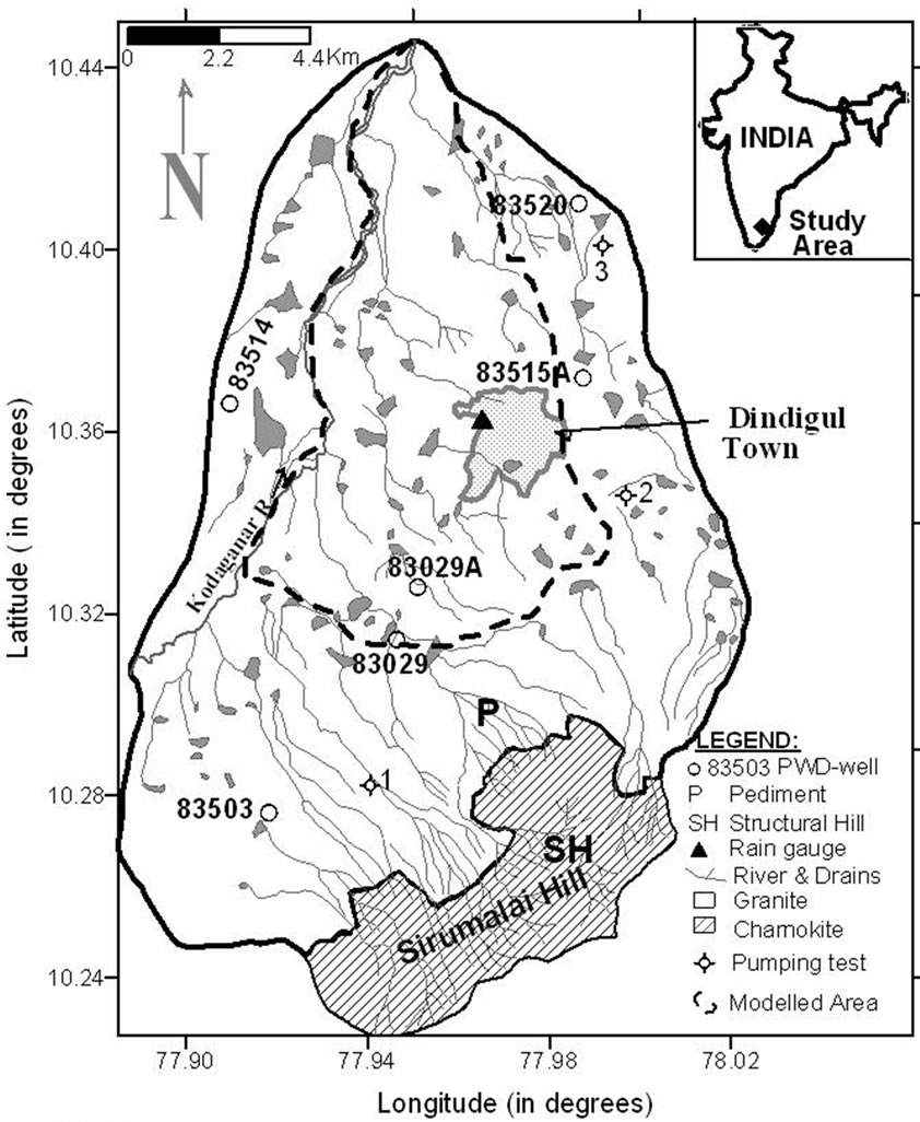
Figure 1. Location map representing the drainage pattern and PWD wells.
by undulating topography with hills located in southern parts, sloping towards north and northeast [6]. The highest elevation (altitude) in the hilly area (Sirumalai Hill) is of the order of 1350 m (amsl), whereas in plains it ranges from 360 m (amsl) in the southern part to 240 m in the northern part. No perennial streams exist in the area, except for short distance streams encompassing 2nd and 3rd order drainage. Runoff from rainfall within the area ends in small streams flowing towards the main Kodaganar River. From a period of 1971-2007 the average annual rainfall is of the order of 905.3 mm. Normally, subtropical climate prevails over the area without any sharp variation. The temperature increases slowly to a maximum in summer months up to May and after which it drops slowly. The mean of the maximum temperature in plains ranges from 36.5℃ to 41.8℃ and in hills, it ranges from 7.9℃ to 21.8℃. The mean of the minimum temperature in plains varies from 17.4℃ to 24℃ and in hills varies from 6℃ to 8.5℃ [1].
2.2. Geological and Hydrogeological Setting
Geologically the area is occupied with Archaean granites and gneisses, intruded by dykes [7]. These formations, including granite, granodiorities, gneissic granite and gneisses, are the most widespread groups of rocks which are mainly composed of gray and pink feldspar with quartz grains, biotite and hornblende [8]. These formations are crossed by sets of joints and fractures, which have also caused weathering of coarser rocks. Weathering occurs due to mechanical and mostly chemical processes that take place, while water in the fractures interacts with the formation. The shallow hard and massive rocks are exposed mostly in the southern part. Another most dominant formation is charnokite, which is found in the extreme southern and southeastern parts of the area (Sirumalai hill) acting as a no flow boundary.
Groundwater occurs mostly in weathered and fractured zones, which are unconfined, semi-confined or confined. The thickness of weather zone varies from 3.1 to 26.6 m but black cotton soil exists in the middle part whereas red sandy soil in northern and southern parts of the study area. It’s thickness varies from 0.52 m to 5.35 m. Such shallow weathered zones may not be stable sources of groundwater for meeting large demands for groundwater [2]. The weathered zone facilitates the movement and storage of groundwater through a network of joints, faults and lineaments, which form conspicuous structural features. Groundwater is extracted through dug well, dug-cum-bore wells and bore wells by bucket & pulley and electric motor methods for different purposes. The shallow aquifer gets both direct recharge from rainfall and indirect recharge as seepage from about 93 irrigation tanks and irrigated fields.
2.3. Methods
Hydrogeological, geophysical and entropy studies were carried out for deciphering subsurface litho zones, understanding prevailing hydrogeological conditions, evaluation of aquifer parameters, such as natural recharge, storativity, and hydraulic conductivity. Groundwater levels were monitored in 6 wells by PWD since 1971, and in addition also collected from 45 and 30 observation wells during April 2001 and February 2009, respectively. To determine aquifer properties, pumping tests were carried out at 3 locations and data was analyzed by numerical methods [9]. A total of 37 Vertical Electrical Soundings (VES) were conducted using Schlumberger electrode configuration for a spread of 60-120 m. Initially VES data had been interpreted through a curve matching technique [10] and then interpreted by computer programme [11]. 6-PWD dug wells were selected for the determination of average natural recharge by the entropy theory [12]. The generated data was utilized in the development of the groundwater flow model. The various steps involved in the modeling in the study are shown in Figure 2.

Figure 2. Flow chart for groundwater flow model.
3. Results and Discussion
3.1. Hydrogeological Investigations
3.1.1. Water Level Measurements
Monthly water level data were available from 6 PWD wells, which are uniformly spread over the study area. A contour map was prepared, from which it was difficult to identify the hydrogeological characteristics of the aquifer with respect to the groundwater flow pattern. The contours don’t follow the topography and drainage patterns. For this reason during April 2001 and February 2009, 45 and 30 water levels were collected and analyzed, respectively. The depth of water table varied from 1.00-22.80 m (bgl) with a mean value of 8.07 m (bgl) in April 2009 and 0.70-17.00 m (bgl) with a mean value of 5.64 m (bgl) in February 2009, because of the variations in weathered thicknesses, intensity of weathering and uneven withdrawal rates. The trend of PWD-well hydrographs closely followed the rainfall trend [6]. In most cases the water level returns to its original position after a good rainfall. This may be due to the rapid recharge taking place due to heavy rainfall and also irrigation return flow [2].
3.1.2. Aquifer properties
Aquifer parameters, namely transmissivity (T) and storativity (S), are vital for groundwater modeling. Several analytical methods have been developed to determine these parameters, however, the numerical approach has an advantage in that it incorporates actual field conditions with ease and hence parameters estimated are more realistic [9]. This method is described in detail by Rushton and Redshaw [13].
During field investigations, 3 existing large diameter open wells fitted with pumps (see Figure 1) were selected for pumping test. Most of these wells had been kept without pumping prior to beginning the test and water levels had been continuously monitored. The period of pumping varied from 45 to 126 minutes, whereas recovery times varied from 170 to 1313 minutes. Both pumping and recovery data were used for interpretation using a forward modeling technique as suggested by Singh [9]. The nearby features, such as water body or lateral inhomogenities had been incorporated into individual interpretations. Initial parameter values were considered to generate time drawdown curves for individual tests, which were then compared with observed timedrawdown/recovery data. The aquifer parameters were varied until a close match was obtained. The best-fit match was considered as representative aquifer parameters. The estimated T and S values varied from 15 to 200 m2/day and 1 × 10⁻⁵ to 3.5 × 10⁻⁴, respectively. It was found within the ranges of T and S values from 4 to 1166 m2/day and 1 × 10⁻⁵ to 9 × 10⁻³, respectively, obtained in Kodaganar River Basin, Dindigul and Karur Districts, Tamil Nadu [2].
3.2. Geophysical Investigations
The resistivity sounding technique [10,14,15] was employed to identify the aquifer geometry. In total 37 Vertical Electrical Soundings (VES) were carried out with current electrode separation of 60-120 m. The curves obtained are classified as A and H-types, which describe the variation in the resistivity of progressive layers below the ground surface. The A and H-type sounding curves reflect the pattern of resistivity distribution with depth. If ρ1, ρ2 and ρ3 are the resistivities of three subsurface layers beginning with ρ1 at the top, then ρ1 > ρ2 < ρ3 is defined as H-type and ρ1 < ρ2 < ρ2 as A-type.
The observed field curves were matched with theoretical master curves to obtain initial parameter values and finally these were used as input in the interpretation of resistivity data through software, namely, RESIST [11]. The interpreted results of VES, when compared with the existing 9 litho-log data [1] and cross-sections of nearby open wells, confirmed the resistivity ranges of different subsurface geo-electrical layers as:
• 2-95 Ω-m: Top soil cover/ clay with kankar
• 6-100 Ω-m: Weathered formation/saturated or saline aquifers
• 100-300 Ω-m: Semi-weathered/fractured granite and gneissic granite
• >300 Ω-m: Hard rock (gneissic granite and gneisses)
The shallow aquifer resistivity in weathered zone ranged from 6.08 to 264.27 Ω-m. The estimated thickness of the weathered zone varied from 5.30 to 26.62 m. It was confirmed that its value ranged from 15.00 to 26.62 m in the western part of Dindigul town. The soil thickness ranged from 0.52 to 5.35 m, whereas the depth of bedrock with weathered thickness: 11.00-26.62 m ranged from 12.00 to 27.67 m (bgl) in western and southwestern parts of the town, which are potentially good groundwater zones.
3.3. Natural Recharge Estimation
For modeling of groundwater resources in the semi-arid area, it is essential to determine natural groundwater recharge. There are several methods for determining groundwater recharge, such as groundwater balance [16]; lysimeters [17]; piston-flow model [18]; RS and GIS techniques [19]; photogeological [20], hydrogeological [21], geophysical methods [22], and 14C-age dating [23]; and regional groundwater models [24]. Among these methods, the tracer technique is one of the best direct methods for estimation of groundwater recharge [18]. This technique estimates recharge on the basis of piston flow model, and has been found useful [25-26]. Other methods are time consuming and sometimes even uneconomical in developing countries, particularly when one has to deal with a large area.
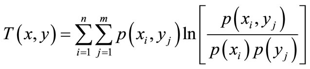
Therefore, an entropy-based approach [12] is developed for assessing natural recharge in this study area. Entropy of a random variable is a measure of the information or uncertainty associated with it. Measures of information include marginal entropy, joint entropy and transinformation. For a random variable x, the marginal entropy, H(x) can be defined as the potential information of the variable. For two random variables x and y, the joint entropy H(x, y) is the total information content contained in both x and y. The mutual entropy (information) between x and y, also called transinformation, T(x, y), is interpreted as the reduction in uncertainly in x, due to the knowledge of the random variable y. It can also be defined as the information content of x that is contained in y. Entropy measures can be expressed using both discrete and analytical approaches [27]. Discrete forms of these entropies can be expressed as:
 (1)
(1)
 (2)
(2)
 (3)
(3)
 (4)
(4)
where x and y are two discrete variables with values xi, ; yj,
; yj,  , defined in the same probability space, each of which has a discrete probability of occurrence p(xi) and/or p(yj) and p(xi, yj) is the joint probability of xi, yj. Note that H(x, y) = H(y, x).
Rainfall is considered as independent random variable (x) and the depth to water table for individual wells as the dependent variable (y). Then, transinformation,  , is interpreted as the reduction in the original uncertainty of depth to water table due to the knowledge of rainfall. It can also be defined as the information content of water table which is also contained in rainfall. In other words, it is the difference between the total entropy and the sum of marginal entropies of these two variables. This is the information repeated in both water table and rainfall, and defines the amount of uncertainty that can be reduced in one of the variables when the other variable is known. On the other hand, marginal entropy, H(x), is defined as the potential information of rainfall. Then, the ratio of
  to H(x) is simply a fraction of recharge due to rainfall. Therefore, the percentage of rainfall, Re (%), contributing to the natural groundwater recharge of an unconfined aquifer is given as [12]:
 (5)
(5)
To determine the fractional amount of rainfall (monitored for 8 years from January 2000 to December 2007 at Dindigul rain gauge station), called natural recharge, marginal entropies and transinformation of rainfall and depth to the water table (collected from 6 PWD wells for the same period, see Figure 1) were calculated. Then a ratio of transinformation to marginal entropy of rainfall was used as a measure for evaluating natural recharge.
Rangarajan and Athavale [28] estimated an average natural recharge ratio 10.11% of seasonal rainfall for 15 different granitic and gneiss areas in varying climatic and
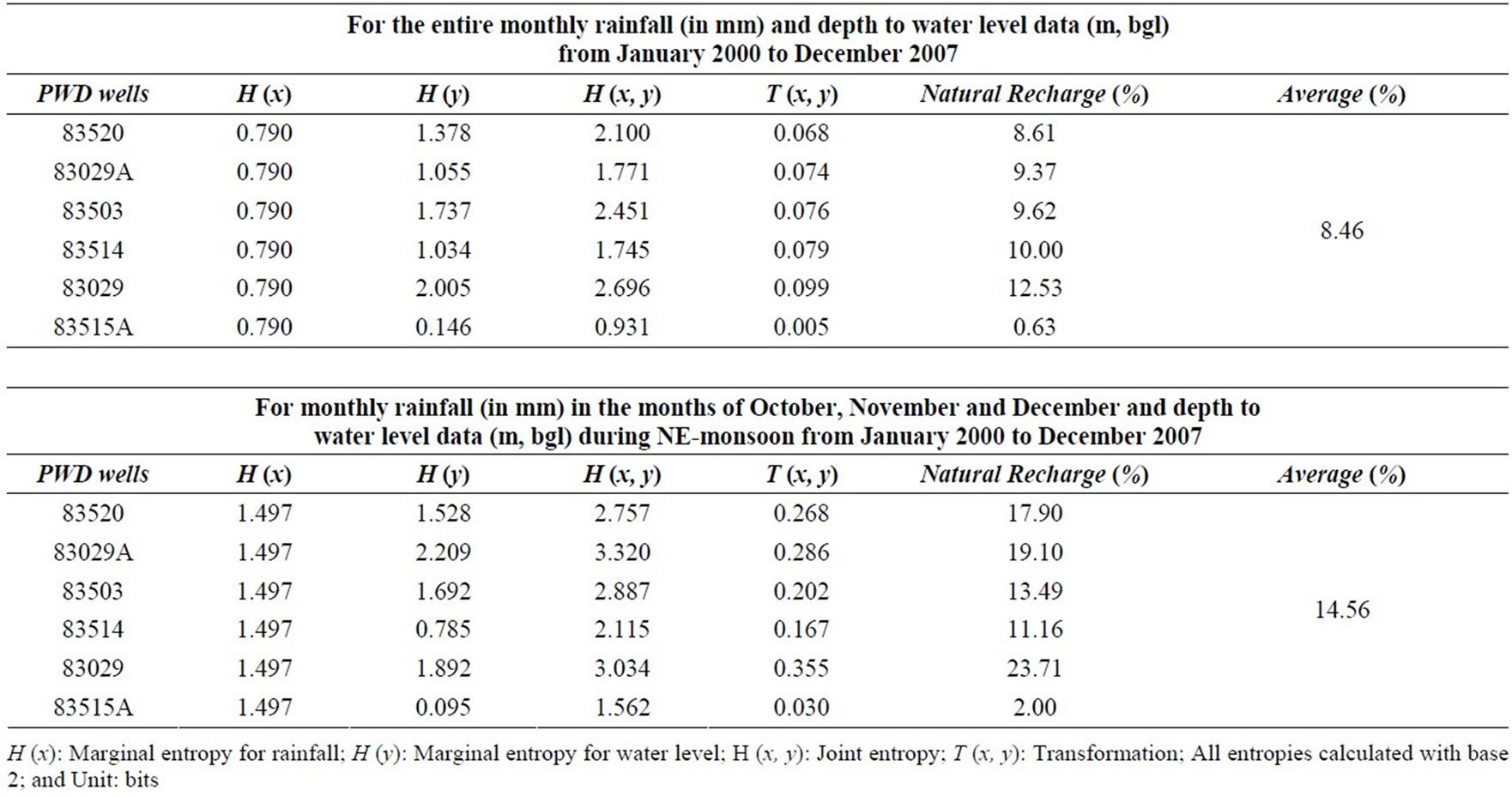
Table 1. Estimated natural recharge using entropy for the entire monthly and NE monsoon data during January 2000 to December 2007.
hydrogeological provinces of India. Out of them, the average recharge ratio was about 9.90% for 4-granitic and gneiss areas in Tamil Nadu state (Southern India). The estimated average natural recharge using entropy varied from 0.63 to 12.53% in the entire period, but it varied from 2.00 to 23.71% only for NE monsoons. The mean of the estimated recharge values was 14.56% of rainfall in NE monsoon (see Table 1).
3.4. Aquifer Modeling
An aquifer model was constructed based upon a conceptual approach. In order to construct the model, boundary condition, grid and time increments were decided, and applied stresses and hydraulic properties were also estimated. Finally, these parameters were tested and adjusted during the calibration procedure, with the intention of reproducing a set of historically observed data. Finally the model was evaluated, considering how reasonably it could represent the actual system.
3.4.1. Conceptualization
The aquifer in the proposed area (see Figure 1) consists mainly of two layers: one-weathered and two-fractured zones of the granite-gneiss formation. The weathered zone overlies the fractured zone (in bedrock), but its thickness varies from place to place. Bedrocks are at a depth of 12.00 to 27.67 m (bgl). The two layers have different hydraulic characteristics and especially the fractured zone has a lower storage coefficient than does the weathered zone. The weathered part of the aquifer was considered as equivalent to a porous zone.
Recharge from rainfall takes place between October and December. The percentage of rainfall that becomes recharge was determined based on the estimated recharge values by entropy [12]. Then it was adjusted during the model calibration. The reason why no recharge takes place between January and September is low rainfall in conjunction high temperature and evaporation. There is no surface water interaction with neighboring sub-watersheds. Groundwater interaction with adjacent area was also considered. The main recharge areas are in the south and southeast, and the main discharge area in the northern part. Thus, groundwater flows southwest, north and northeast. Kodaganar River acts as the main drainage route and flows north. However, it flows only during the wettest months of the year (October-December). The aquifer seems to be in interaction with the river and probably the water table is higher than the river stage. In order to satisfy irrigation, domestic and industrial needs, increasing groundwater abstractions take place in the area. Industrial and domestic abstractions are about 20% of the total abstracted volume. Irrigation abstractions most likely occur during the dry period (January to September).
3.4.2. Model Design Approach
A single layer model of the tannery belt (see Figure 1) was selected and a groundwater flow regime was prepared for the following reasons: 1) geometry of fractured zone was unknown, 2) no data existed about the actual amount of abstractions that takes place in this fractured zone, and 3) the number of abstracting wells reaching the fractured zone was unknown. The geometry and boundary conditions are generally complex. Analytical methods are rarely applicable for determining a closed form solution of the partial differential equations of 2-D groundwater flow equation [13] as given below:
 (5)
(5)
where Kxx & Kyy are the hydraulic conductivities along the x & y directions, h is the hydraulic head, Ss is the specific storativity, W is the groundwater volume flux per unit area (positive for outflow and negative for inflow), and x and y are the Cartesian coordinates.
Equation (5) was solved using a finite difference approximation technique. The starting point for the application of this method was discretization of modeled area into small grid form. This leads to set of simultaneous algebraic equations, which was solved using the Visual MODFLOW Premium 4.4 modeling code. This code has been widely used and is accepted to produce numerically stable solutions. The method selected for the numerical solution of the algebraic equation set is WHS.
3.4.3. Grid Design
In order to set up the model in MODFLOW set of codes, the area of interest (an area: 75.56 km2) was divided into a series of grid blocks or cells (see Figure 3), a grid size of 250 m × 250 m (total grids = 1209) and it would be used for mass transport modeling as the hydrochemical data is available in this part. The elevation of the top of shallow aquifer varied from 232.00 to 314.00 m (amsl), while the bottom from 220.00 to 306.00 m (amsl). Both the top and bottom elevations of the aquifer were defined with respect to above mean sea level (amsl) in grid form with the use of SURFER v.8.0 using the kriging method and converted into ASC-format, which was imported into the model under the MODFLOW environment. The variation of aquifer thickness for a typical row number 44 is shown in Figure 4. The layer had the confined/ unconfined condition and corresponded to a layer type 2 in Visual MODFLOW Premium 4.4.
3.4.4. Boundary Conditions
Generalized head boundary: The southern and eastern boundaries of the modeled area were simulated through a generalized head boundary (GHB) in order to represent the groundwater inflow and outflow through nearby sub-watersheds [29]. The values that were used in the steady state simulation in this model were obtained by
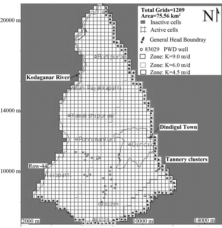
Figure 3. Grid map and hydraulic conductivity distribution of the tannery belt.

Figure 4. Simulated vertical cross section along row number 44.
calibration and were kept constant throughout the transient simulation, because there existed no data at all for this boundary. The values, that were finally used, were boundary conductance of 5.2 × 10³ m2/d and head 4 m (bgl) at or beyond the boundary.
River : Kodaganar River is a special case of a headdependent boundary. It was simulated through a river boundary condition. The properties were set for each river cell boundary as: the river stage (5 m below ground surface), riverbed bottom (4 m below the river stage), riverbed thickness (1.0 m), riverbed vertical hydraulic conductivity (Kz = 2.0 m/d) and river width (10 m). Because there were no data at all for Kodaganar River, the properties were set through the conditional process.
3.4.5. Hydraulic Parameters
Initially the results from the only available aquifer test were used as the hydraulic properties of the aquifer. However, these proved to be inadequate to represent the whole system, which was complicated and heterogeneous due to the presence of weathered zone. Hence various property zones were assigned, and their values were adjusted during calibration.
3.4.5.1. Hydraulic Conductivity The final distribution of hydraulic conductivity zones is illustrated in Figure 3. The southern part was assigned a conductivity value of 4.5 m/d, in the central part 6 m/d and northern part 9 m/d.
3.4.5.2. Specific Yield The final distribution of specific yield, as indicated by the model calibration, was assigned. The southern part was assigned a specific yield value of 0.015, the central part 0.02, and the northern part 0.03. Similarly specific storages of 0.00005, 0.0012 and 0.0002 were assigned to these zones, respectively. The effective porosity and total porosities were also assigned uniformly throughout the area as 2.75% and 3.00%, respectively [30-31].
3.4.6. Applied Stresses
3.4.6.1. Abstractions The main groundwater application in the area is irrigation using 80% of the total abstracted volume. The remaining 20% of the abstraction is reserved for domestic and industrial uses [1]. Irrigation abstractions are spread out in the area (except on the hills), while the domestic/industrial abstractions are assumed to be concentrated around towns and the villages. However, all well locations were unknown in the tannery belt. Therefore, the known location of 96 wells, which were used for domestic, industrial and irrigation abstractions, were used to simulate abstractions, because the total abstracted volume was about 23, 588 m3/day in 2000 [1]. The abstractions during subsequent years had to be estimated by increasing 3% every year. Abstractions from each irrigation and domestic/industrial wells were used for steady, transient and prognostic models.
3.4.6.2. Recharge Recharge was separated into recharge from rainfall and recharge from irrigation return flows. Recharge from rainfall and irrigation return flows occurs during the wet period (October-December) in the study area, whereas recharge only from irrigation return flows occurs during the dry period (January-September). Initially as recharge, a percentage (2.00-23.71%) of the rainfall was used as a direct rainfall recharge in the model, although this approach proved to underestimate during transient calibration due to its spatial variability and the computed water level values were comparatively lower than the observed ones. Therefore, a higher percentage of rainfall (12-37%) was used (see Figure 5) for understanding the combined effect of natural recharge and irrigation return flows in the study area. Then the evapotranspiration package was added to the system for the dry period (January-September) only. During the wet period evapotranspiration was insignificant, and therefore it was set to zero.
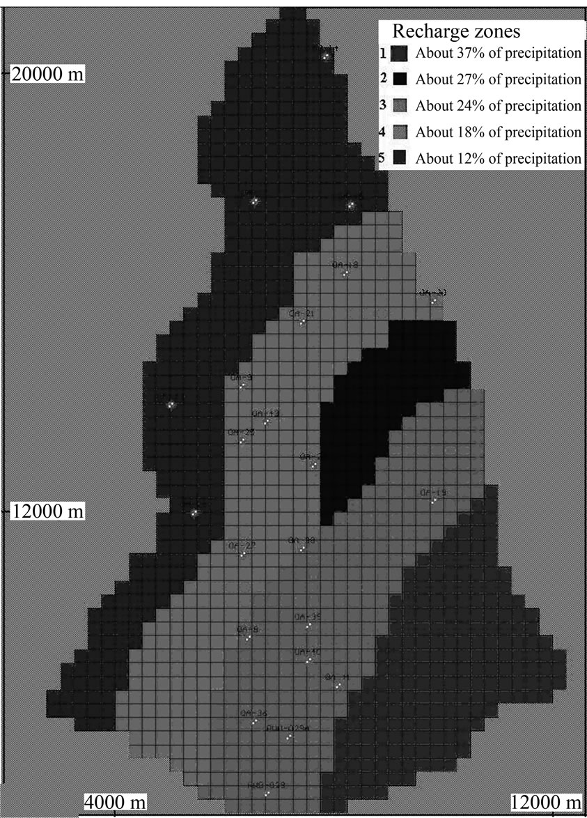
Figure 5. Recharge distribution in the groundwater flow model.
Evaporation was estimated to a maximum rate of 52.5 mm/ year for a depth of up to 3 m based on the type of soil, crops and plants that grow in the area. This way, evapotranspiration occurred when the water table was within 3 m from the ground surface, i.e., the evapotranspiration rate was zero 3 m below the ground surface and 52.5 mm/year at the ground surface. Finally, irrigation return flows were estimated at about 4-38% of the abstracted volume and added to the aquifer system. Based on hydrogeological and climate conditions prevailing in the area, the recharge values of 80, 120, 160, 180 and 250 mm/year, respectively, were assigned to zones 1-5, as shown in Figure 5.
3.4.7. Model Calibration
The purpose of model calibration was to estimate the acute parameters for the given boundary conditions and stresses within a certain established range of error (calibration targets). In this study a trial and error calibration was used. Parameters were initially assigned to each node in the grid. Then these parameter values were adjusted sequentially to match the calibration targets. The calibration parameters, set in the model, were the generalized head boundary, recharge, evapotranspiration, hydraulic conductivity, and specific yield.
3.4.7.1. Calibration Stages Model calibration was performed in three stages: 1) steady state, 2) transient state, and finally 3) prognostic model under transient state. The purpose of the steady state calibration was to provide a set of initial conditions for the transient model and initial estimates of the calibration parameters, which would be further calibrated during the transient calibration.
The data available for model calibration existed for the period April 2001-February 2009. Since the estimated abstraction for the year 2001 was not zero, no steady data existed. Therefore, the calibration of a dynamic steady state model was considered in order to obtain an initial head distribution for April 2001. The calibrated parameter values were imported into the transient model for the period April 2001 to February 2009. The calibration parameters were further adjusted in the transient model and they were imported back in the steady state model, in order to reproduce the corresponding new initial conditions. Finally the new initial conditions were imported once more in the transient model as well as the prognostic model, and this calibration was at least improved by the execution of sensitivity analysis.
3.4.7.2. Calibration Criteria Each grid cell had a 5 m difference at the top of the aquifer as well as approximate 5 m difference in the head from the adjacent ones. Each monitoring well could be anywhere within the same cell. Therefore the error due to space discrimination allowed in the steady state calibration targets ±2.5 m [29]. Similarly, because it was not known when within a month the observation measurements were taken, the error due to time discrimination was ±0.5 m. However, in transient calibration errors larger than ±2.5 m were allowed, considering the size of the area and grid, and in fact abstractions were completely unknown, especially for early simulation years. During transient calibration the main idea was to match the trends in the hydrographs reproduced at two PWD wells. But the numerical round off error was evaluated by examining the water mass balance calculated by the model. This error should ideally be less than 0.1% [32] and was tested for both the steady state and transient models.
3.4.7.3. Steady State Calibration The steady state simulation had been performed for averaged rainfall and abstraction values for the period April 2001 to March 2002. The model was run for 365 days. The estimated abstractions for these months were added and divided by 365 to get an average constant daily rate. Similarly, rainfall during the wet months was also added and divided by 365 to get an average daily value for this period. This model was calibrated against the general head boundary, recharge, evapotranspiration and hydraulic conductivity through a sequence of sensitivity analysis runs, starting with the parameters for which the least data were known. The values were adjusted during trial and error runs, aiming at the smallest sum of squares of residual errors in the targets.
The steady state model was calibrated against 22 head values observed in April 2001. The calibrated water level at the targets varied from 225.91 to 277.96 m (amsl) with a mean of 255.66 m (amsl). It showed that groundwater was flowing towards the river from the tannery clusters. The computed vs. observed heads with statistical analysis of the steady state calibration results are shown in Figure 6. The model was considered as sufficiently calibrated as 82% of the targets satisfied the ±2.5 m criterion. Four targets showed high residual errors with a maximum value of 5.26 m (see Figure 6) but these can be justified. Target OA-15 was towards the northern boundary for which there was no data available. Targets OA-22 and 41 were being completely controlled by the abstractions. The GHB was controlling the target 83029. Finally, the numerical error in the model was minimal, since the mass balance error was 0.0108%, as shown in Table 2. The table shows that groundwater abstraction was about 80.43% of annual groundwater recharge, but 10.25% of the annual recharge was being used up by evapotranspiration. There was a combination of inflow and outflow for river leakage. But the outflow of river leakage was comparatively higher than inflow, which was about 3.17% of the annual groundwater recharge. In

Figure 6. Computed vs. observed heads in the steady state calibration (April 2001).
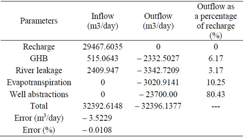
Table 2. Steady state calibration mass balance results (m3/day).
this steady state, the minimum and maximum groundwater velocities were calibrated in order of 0.01 and 0.83 m/d with a mean of 0.29 m/d and it varied from 0.21 to 0.41 m/d in the tannery cluster.
3.4.7.4. Transient Calibration The transient model was simulated for the period between April 2001 and February 2009, using initial heads computed in April 2001 under the steady state model. Each year in the transient model was divided into 4 stress periods: one dry period, which lasts 270 days and has 9 stress periods–one for each simulated month; and three distinct 30 days wet periods, one for each recharge month (i.e., October, November & December). This was done with the objective of better simulating the difference in rainfall and consequently in recharge between the three wet months. Each stress period was divided into 10-time steps in order to make it easier for the model to converge. In total there are 95-stress periods with 950 time steps in the transient model. The results of sensitivity analysis, summarized in Figure 7, shown that the model was insensitive to the recharge in the zone-5 and specific yield in the zone-3 due to the presence of Kodaganar river, as there was almost no change in the RMS error for a quite large change in the parameter multipliers. Nevertheless the model was sensitive to all the other calibration parameters in the different zones (recharge, hydraulic conductivity, specific yield and slightly evapotranspiration). Sensitivity analysis showed that even lower values in the evpotranpiration rate minimized the error. The recharge and hydraulic conductivity values used, on the other hand, gave the smallest RMS errors. Although the curves in Figure 7 indicated the use of lower evpotranpiration rate, the latter was not changed due to the fact that calibrated and observed heads matched sufficiently closely. In the transient model of dry stress period the evapotranspiration rates reduced to 73.4 m3/d in 2008 from 250.1 m3/d in 2001 due to decline of groundwater level in the study area.
Computed versus observed heads for each calibration target, during all time steps considering a total of 243 observed data points in the entire simulation show that maximum and minimum residuals were –18.93 m and 0.027 m observed at well OA-40 in April 2001 and PWD well 83029, respectively, with RMS = 6.756 m in the transient calibration statistics. The numerical error is order of ±0.0032% in the water mass balance during the model run. Two representative well hydrographs (in which only historical data were available) reproduced by the transient model in the calibration targets. It could be observed from the well hydrographs that the model effectively simulated groundwater flow in the central and northern parts. In the southern part however, the water table hydrograph was continually noticeably lower than observed values (i.e., hydrographs at PWD wells 83029 and 83029A), but their trends were similar to observed hydrographs, which was controlled by GHB.
The groundwater head distribution for February 2009 (see Figure 8) was reproduced using the transient model (at the stress period 95). It shows that groundwater was moving towards NW from the tannery cluster and NE in the northern part of the area. In this period computed and observed heads had a RMS error of 3.29 m for 20 targets with a correlation coefficient of 0.979. In February 2009, the minimum and maximum groundwater velocities were 0.02 and 0.91 m/d with a mean of 0.34 m/d (see Figure 9). The calibrated groundwater heads varied from 239.14 to 286.02 m (amsl), whereas observed heads from 240.94

Figure 7. Results of sensitivity analysis for the transient model.
to 289.28 m (amsl) in the study area. The velocity varies from 0.32 to 0.52 m/d in the tannery cluster.
3.4.7.5. Predictive Model The transient model was used to perform predictive simulations in order to assess the sustainability of groundwater system. Although a predictive simulation could last up to twice the calibrated period [29], it was decided in this case to simulate for 6 years in the future, instead of 16, because of the high uncertainty in predicting future hydraulic conditions and stresses to the system. Hence predictive simulations were performed for the period between March 2009 and December 2015.
1) Extrapolation of past and present stresses to future Similar to the transient model, each year was divided into a dry stress period (January-September) and three wet periods (i.e., October, November and December). The extrapolation of rainfall and abstractions to the future was being discussed.
Rainfall and recharge: The generation of future rainfall values would require extensive statistical analysis. Since the objective of this study was not to predict exactly what will happen in the future but to examine the sustainability of the system it was decided to generate future rainfall values by simply replicating the past and present rainfall pattern. Since rainfall for the year 2001-2007 was known, the same value was repeated once more for the wet months until year 2015. Then recharge from rainfall was calculated using the same percentages as in the transient model.
Abstractions: Prediction of groundwater demands in future would require a socio-economic study, which is beyond the scope of this study. Since the main objective was to examine the response of the aquifer under different abstraction stresses, predictive simulations were performed under four different schemes, i.e., in Scheme I: abstraction was completely stopped; Scheme II: abstraction was kept at a current rate of year 2009; Scheme III: abstraction was increased by about 10%; and Scheme IV: 20% of the abstraction in 2009 was for domestic/Industrial and irrigation purposes.
2) Prediction Model It was presumed that the aquifer would receive the same recharge just like the previous 6 years, while the abstraction for domestic/industrial usages was kept zero meaning there is no abstractions throughout the area. The calibrated well hydrographs are indicated a progressive

Figure 8. Groundwater head distribution (produced by the transient model) in Feb. 2009.
increase of water level. The increased water table varied from 0.09 to 14.29 m from March 2009 to 2015. Maximum changes were observed on the eastern side and minimum towards the river. In Scheme II, the abstraction was kept constant in year 2009. The computed well hydrographs indicated a slow decline of the water table. It varied from –0.001 to –0.89 m with an average decline of 0.23 m throughout the area, but the changes of water level were almost zero along the river side. When the abstraction was increased by 10% of abstraction in 2009, then well hydrographs declined from –0.009 to –2.28 m (see Figure 10(a)). But in the case of increased abstraction of 20% in year 2009, the water level declined comparatively more. The changes of water level varied from –0.02 to –3.74 m (see Figure 10(b)). This decline would take place at an alarming rate with a significant decline of 1.49 m within 6 years.
In order to explore the possibility of increasing the groundwater level in this area through various means such as artificial recharge, the net recharge in the model
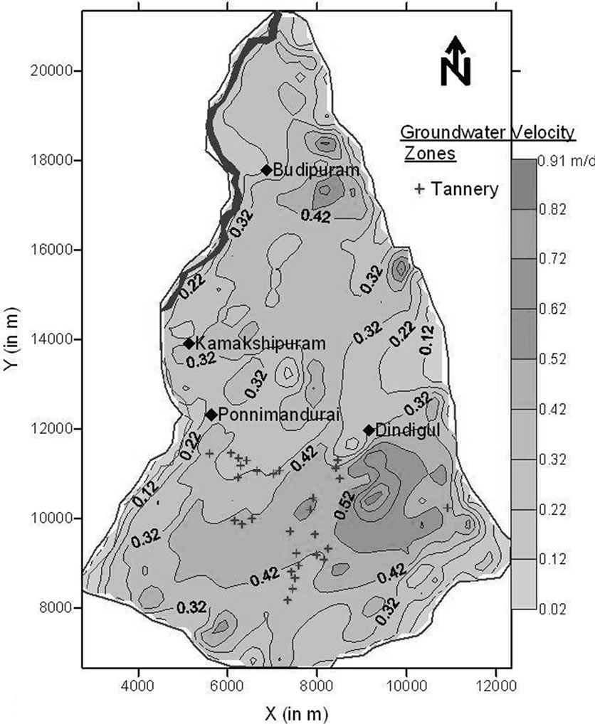
Figure 9. Groundwater velocity distribution in February 2009.
was increased, keeping in view the groundwater potential recharge areas. The abstraction rate was kept same as in Schemes III & IV. It was found that even at a moderate rate of increase in recharge, the groundwater level in many areas would rise in both the schemes.
4. Conclusions
Groundwater flow model was simulated for a tannery belt in Southern India by assigning input and output stresses. The simulated results show the following:
• Groundwater flows towards northwest in the southern part, and north and northeast in the northern part of the study area. In the tannery cluster the groundwater velocity varies from 0.21 to 0.41 m/d in April 2001 and 0.32 to 0.52 m/d in February 2009, which is important for mass transport modeling.
• The estimated average groundwater recharge is about 80-250 mm/year, which is equivalent to 12-37% of annual rainfall. The total groundwater abstraction is about 80.43% of annual groundwater recharge, but 10.25% is being used up by evapotranspiration.
• Groundwater velocity is more sensitive to recharge from rainfall, hydraulic conductivity, and specific yield.
• The shallow aquifer, without further decline in water
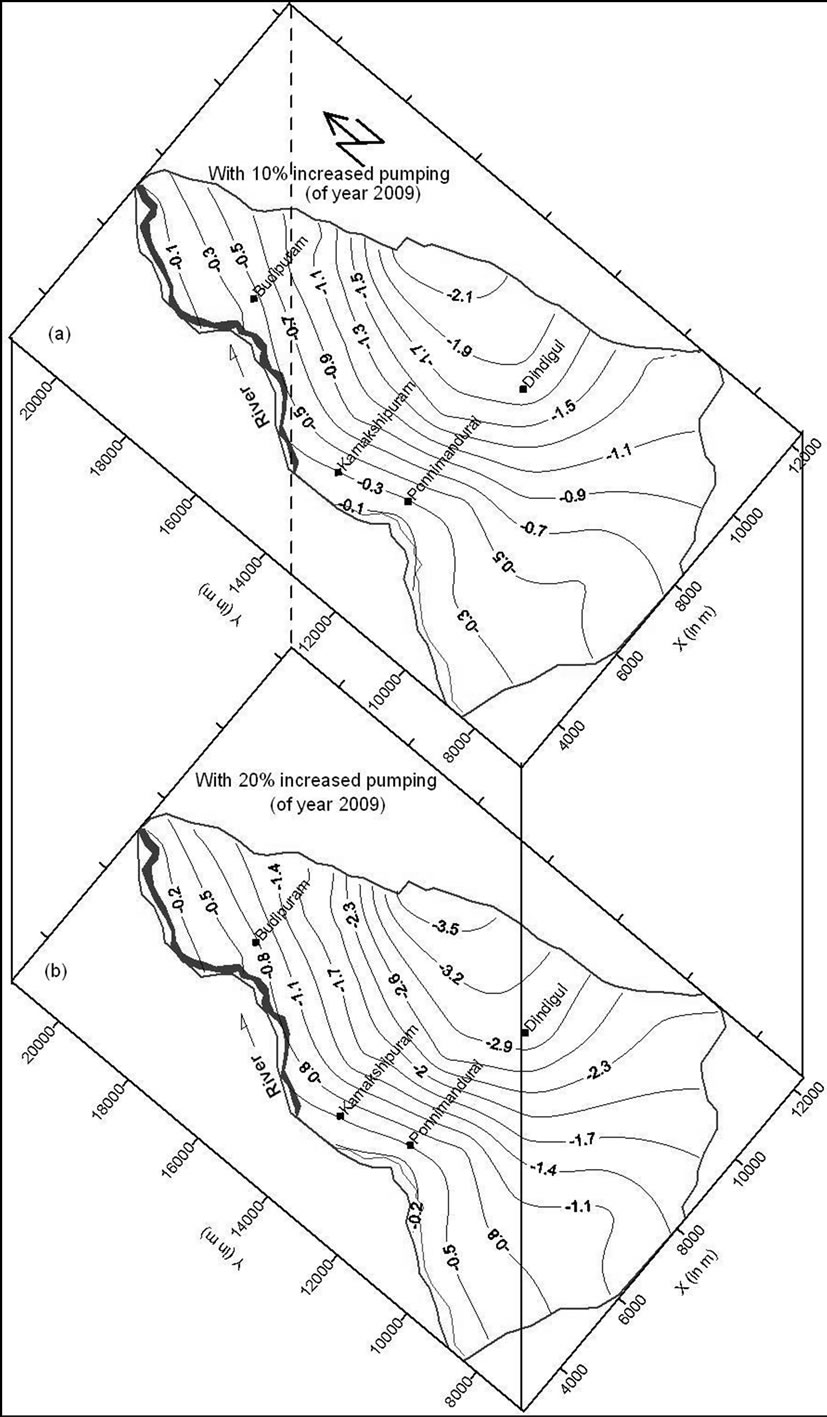
Figure 10. Groundwater level changes from March 2009 to 2015 (a) with 10% increasing and (b) 20% increasing pumping of 2009.
level, can sustain a pumping rate of 24892 m3/day under a certain constraint. Any additional increase of withdrawal from this aquifer would result in a progressive decline of water level.
It is, therefore, suggested that groundwater resources be augmented through artificial recharge methods. As a first step, removal of silt in the existing irrigation tanks will considerably improve vertical infiltration, and construction of check dams in the upland area will enhance recharge. The present model is only a preliminary one and the obtained information represents a base for future groundwater work that will help in the planning, protection and decision-making regarding the groundwater management in this area. But it should be updated with additional field data. Then optimal utilization schemes can be evolved.
5. Acknowledgements
This work was performed, in part, under the BOYSCAST Fellowship of the first author (Dr. N. C. Mondal) funded by Department of Science & Technology (Government of India), New Delhi (Ref. No. SR/BY/A-05/ 2008, Date: 16-19th January 2009). The officers of PWD, Chennai provided suitable data and the members of Groundwater Division, NGRI helped during the field work. The authors are thankful to them.
REFERENCES
- Public Works Department, “Groundwater Perspectives: A Profile of Dindigul District, Tamilnadu,” PWD (Governmentt of India) Reptort, Chennai, 2000.
- V. S. Singh, N. C. Mondal, R. Barker, M. Thangarajan, T. V. Rao and K. Subramaniyam, “Assessment of Groundwater Regime in Kodaganar River Basin (Dindigul district), Tamilnadu,” Technical Report, 2003.
- N. C. Mondal, V. K. Saxena and V. S. Singh, “Assessment of Groundwater Pollution Due to Tanneries in and around Dindigul, Tamilnadu, India,” Environmental Geology, Vol. 48, 2005, pp. 149-157. doi:10.1007/s00254-005-1244-z
- N. C. Mondal and V. P. Singh, “Need of Groundwater Management in Tannery Belt: A Scenario about Dindigul Town, Tamil Nadu,” Journal of the Geological Society of India, Vol. 76, 2010, pp. 303-309.
- M. G. McDonald and A. W. Harbaugh, “A Modular Three-Dimensional Finite Difference Ground-Water Flow Model,” U.S. Geological Survey Techniques of Water-Resources Investigations, Book 6, Chapter A1, 1988, p. 586.
- N. C. Mondal and V. S. Singh, “A New Approach to Delineate the Groundwater Recharge Zone in Hard Rock Terrain,” Current Science, Vol. 87, 2004, pp. 658-662.
- R. Chakrapani and P. M. Manickyan, “Groundwater Resources and Developmental Potential of Anna District, Tamil Nadu State,” CGWB Report, Southern Region, Hyderabad, India, 1988, p. 49.
- M. S. Krishnan, “Geology of India and Burma,” CBS Publishers and Distributions, India, 1982.
- V. S. Singh, “Well Storage Effect during Pumping Test in an Aquifer of Low Permeability,” Hydrological Science Journal, Vol. 45, 2000, pp. 589-594. doi:10.1080/02626660009492359
- E. Orellana and H. M. Mooney, “Master Tables and Curves for Vertical Electrical Sounding over Layered Structures,” Interciencia, Madrid, Spain, 1966.
- B. Vander Velpen, “RESIST: a Computer Processing Package for DC Resistivity Interpretation for the IBM PC and Compatibles,” M. Sc. Thesis, ITC-Delft, The Netherlands, 1988.
- N. C. Mondal and V. P. Singh, “Entropy-Based Approach for Estimation of Natural Recharge in Kodaganar River Basin, Tamil Nadu, India,” Current Science, Vol. 99, No. 11, 2010, pp. 1560-1569.
- K. R. Rushton and S. C. Redshaw, “Seepage and Groundwater Flow,” Wiley, Chichester [Eng.], New York, 1979.
- Compagnie General de Geophysique, “Master Curves for Electrical Sounding,” European Association of Exploration Geophysicists (EAEG), The Hague, 1963, p. 49.
- P. K. Bhattacharya and H. P. Patra, “Direct Current Geoelectric Sounding-Principles and Interpretation,” Amsterdam, Elsevier, 1968.
- C. W. Fetter, “Applied Hydrogeology,” Prentice Hall, Inc. New York, 2001.
- J. C. Nonner, “Introduction to Hydrogeology,” IHE Delft Lecture Notes Series, Taylor and Francis, London, 2006, p. 258.
- U. Zimmermann, K. O. Munnich and W. Roether, “Downward Movement of Soil Moisture Traced by Means of Hydrogen Isotopes,” American Geophysical Union, Geophysical Monograph Series, Vol. 11, 1967, pp. 28-36.
- V. M. Chowdary, D. Ramakrishnan, Y. K. Srivastava, V. Chandran and A. Jeyaram, “Integrated Water Resource Development Plan for Sustainable Management of Mayurakshi Watershed, India Using Remote Sensing and GIS,” Water Resource Management, Vol. 23, 2009, pp. 1581-1602. doi:10.1007/s11269-008-9342-9
- R. B. Salama, I. Tapley, T. Ishii and G. Hawkes, “Identification of Areas of Recharge and Discharge Using Landsat-TM Satellite Imagery and Aerial-Photography Mapping Techniques,” Journal of Hydrology, Vol. 162, No. 1-2, 1994, pp. 119-141. doi:10.1016/0022-1694(94)90007-8
- P. Raj, “Trend Analysis of Groundwater Fluctuations in a Typical Groundwater Year in Weathered and Fractured Rock Aquifers in Parts of Andhra Pradesh,” Journal of the Geological Society of India, Vol. 58, 2001, pp. 5-13.
- D. Muralidharan and G. B. K. Shanker, “Various Methodologies of Artificial Recharge for Sustainable Groundwater in Quantity and Quality for Developing Water Supply Schemes,” In: Proceedings of the All Indian Seminar on Water Vision for the 21st Century, IAH, Jadavpur University, Kolkata, 2000, p.208-229.
- D. B. Bredenkamp and J. C. Vogel, “Study of a Dolomitic Aquifer with Carbon-14 and Tritium,” In: Isotope Hydrology, Proceedings Symposium of International Atomic Energy Agency and UNESCO, Vienna, March 1970. Vienna, International Atomic Energy Agency STI/PUB/255, Paper No SM-129/21, 1970, pp. 349-372.
- T. Sibanda, J. C. Nonner and S. Uhlenbrook, “Comparison of Groundwater Recharge Estimation Methods for the Semi-Arid Nyamandhlovu Area, Zimbabwe,” Hydrogeology Journal, Vol. 17, 2009, pp. 1427-1441. doi:10.1007/s10040-009-0445-z
- R. Chand, G. K. Hodlur, R. Ravi Prakash, N. C. Mondal and V. S. Singh, “Reliable Natural Recharge Estimates in Granite Terrain,” Current Science, Vol. 88, 2005, pp. 821-824.
- R. Rangarajan, N. C. Mondal, V. S. Singh and S. V. Singh, “Estimation of Natural Recharge and Its Relation With Aquifer Parameters in and around Tuticorin Town, Tamil Nadu, India,” Current Science, Vol. 97, 2009, pp. 217-226.
- V. P. Singh, “Entropy Based Parameters Estimation in Hydrology,” Kluwer Academic Publishers, Boston, 1998.
- R. Rangarajan and R. N. Athavale, “Annual Replenishable Groundwater Potential of India - An Estimate Based on Injected Tritium Studies,” Journal of Hydrology, Vol. 234, 2000, pp. 38-53. doi:10.1016/S0022-1694(00)00239-0
- M. P. Anderson and W. Woessner, “Applied Groundwater Modeling-Simulation of Flow and Advective Transport,” Academic Press, San Diego, USA, 1992.
- K. R. Rushton and J. Weller, “Response to pumping of a weathered-fractured granite aquifer,” Journal of Hydrology, Vol. 80, 1985, pp. 299-309. doi:10.1016/0022-1694(85)90123-4
- Groundwater Resource Estimation Committee (GREC), “A Report on Ground Water Resource Estimation Methodology-1996,” Ministry of water resources (Government of India), 1996.
- L. F. Konikow and J. D. Bredehoeft, “Computer Model of Two-Dimensional Solute Transport and Dispersion in Groundwater,” Techniques of Water-Resources Investigations of the USGS; Chapter C2, Book 7, 1978, p. 90.