Technology and Investment
Vol.2 No.4(2011), Article ID:8355,11 pages DOI:10.4236/ti.2011.24024
An Efficient and Concise Algorithm for Convex Quadratic Programming and Its Application to Markowitz’s Portfolio Selection Model
1School of Management, Wuhan University of Technology, Wuhan, China
2Institute of Applied Informatics and Formal Description Methods (AIFB), Karlsruhe Institute of Technology (KIT), Karlsruhe, Germany
E-mail: zhangzz321@126.com, huayu.zhang@kit.edu
Received May 16, 2011; revised September 9, 2011; accepted September 16, 2011
Keywords: Convex Quadratic Programming, Mean-Variance Portfolio Selection Model, Pivoting Algorithm
Abstract
This paper presents a pivoting-based method for solving convex quadratic programming and then shows how to use it together with a parameter technique to solve mean-variance portfolio selection problems.
1. Introduction
There are a variety of algorithms for solving convex quadratic programming (QP). The most well-known one is active set method [1,2]. However this method is difficult to learn for many people due to its operational manner. In this paper we present a pivoting-based method for solving convex QP which is efficient for calculating and concise for understanding.
The Karush-Kuhn-Tucker conditions (KKT conditions) of QP is a system of (in) equalities where all the expressions are linear equalities or inequalities except for complementarity conditions. Like Wolfe’s method [3] we solve the linear part by a kind of pivoting operation while maintaining the complementarity conditions in the computational process. However the system computed by our method has a much smaller size because many variables are deleted from the KKT conditions.
In 1952 Harry Markowitz published the milestone paper “Portfolio Selection” in which the portfolio selection problem is formulated as a convex quadratic program with nonnegative variables [4,5]. It is nearly 60 years. However most people still think the model is difficult to solve and few people conduct their investment activities by calculating efficient portfolios for references. We see that every investments textbooks have a figure to show portfolios which are formed by two assets with different correlation coefficients. But we can hardly see a book which has an example to show portfolios formed by three or more assets in the case of no short sale. We will present a pivoting-based algorithm together with a parameter technique to solve Markowitz’s portfolio selection model in a very simple form. The most important advantage of our parameter technique is that it can continuously obtain minimal risk portfolios at different levels of return in linear time after a portfolio is established by the pivoting algorithm.
The rest sections of this paper are organized as follows. In Section 2, we introduce a pivoting-based algorithm for solving the system of linear inequalities and the parameter technique for generating new basic solutions which are associated with different right-hand side terms. In Section 3, we introduce basic concepts and operations for solving the convex QP. In Section 4, we discuss how to solve Markowitz’s mean-variance portfolio selection model. For brevity, relative theorems and proofs as well as tedious reasoning processes are omitted. For details, the reader refers to [6-8].
2. The System of Linear Inequalities
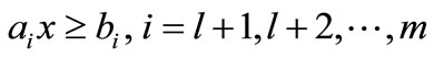
Consider a system of linear inequalities in the form:
 (2.1)
(2.1)
where ,
,  and bi is a scalar,
 .
.
In our algorithm, the following concepts are employed.
A set of maximum linearly independent vectors of a1, a2,  , am is called a basis of (2.1). Vectors in the basis are called basic otherwise called nonbasic. The equalities and inequalities associated with basic vectors are called basic otherwise called nonbasic. The system of basic (in) equalities is called a basic system and whose solution set is called a basic cone. The solution to the system of equations that are corresponding to basic (in) equalities, i.e., the vertex of the basic cone, is called basic solution.
Geometrically, our algorithm begins with a basic cone whose vertex is denoted by . If
. If  lies on the hyper-planes determined by every equalities and lies in the half-spaces determined by every inequalities of (2.1), it is a solution to the entire system. Otherwise there exists an inequality (or equality) such as
  so that
  which is called a violating inequality against
 . If the intersection of the half-space
  and the basic cone is empty, there is no solution for (2.1). Otherwise
  is projected onto the boundary
  of the half-space where
  replaces a basic inequality to constitute a new basic cone. Then the same process is repeated.
Algebraically, a nonbasic (in) equality replacing a basic inequality is accomplished by the following pivoting operation.
Given a basis of (2.1), let I0, I1, I2 and I3 be the index sets for basic equalities, basic inequalities, nonbasic inequalities and nonbasic equalities respectively. Let  be the basic solution, i.e.,
  ,
, . Suppose that
 (2.2)
(2.2)
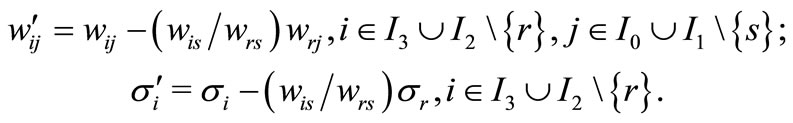
If wrs ¹ 0 for an r Î I3ÈI2 and an s Î I1, from the rth expression of (2.2) we have
 (2.3)
(2.3)
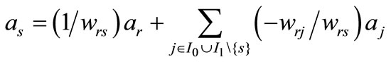
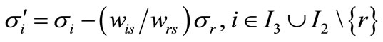
Substitute it into the other expressions of (2.2) to yield
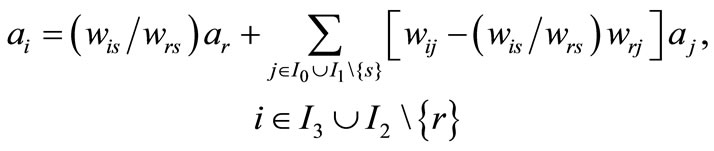 (2.4)
(2.4)
Now, we have a new basic cone whose index set is  and the associated basic solution is denoted by
 . Multiply both sides of (2.4) by
  on the right to have
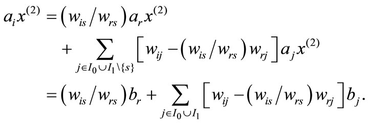
Multiply both sides of (2.2) by  to have

Therefore
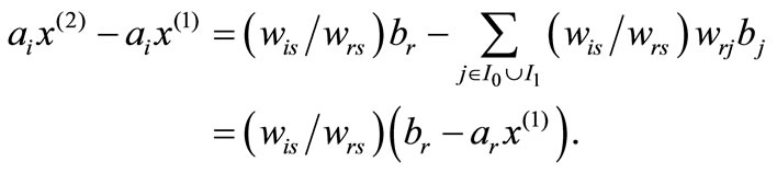
Rewrite the above expression as
and let ,
,  ,
,  to have
 .
.
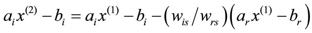
In the same way, from (2.3) we have
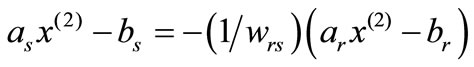
or
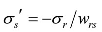 where
where .
.
The above operational process is called a pivoting (operation) and wrs is called pivot (element). The row of wrs is called pivot row and the column of wrs is called pivot column. We say ar enters and as leaves the basis and the exchange of these two vectors is denoted by ar ↔ as. The process is simply shown by Tables 1 and 2.
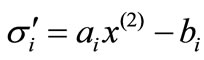
Where
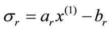
For Table 1,  is called the deviation of ai or the associated (in-) equality with respect to
 . If
. If  ;
;  then
then  is a solution to system (2.1). If
 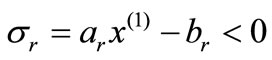 for some r Î I2,
  is called

Table 1. Initial table.
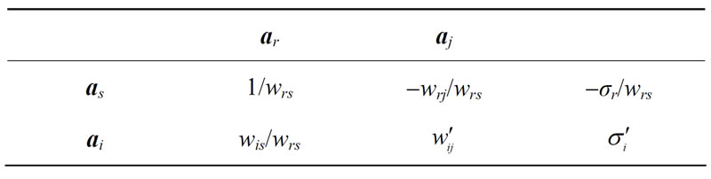
Table 2. The result of pivoting.
violating inequality against  and
and  is called the distance from
  to
to .
.
The computational steps for the system of linear inequalities are as follows.
Algorithm 2.1. Pivoting algorithm for system (2.1).
Step 1. Construct initial table.
If (2.1) has an inequality in the form of ,
,  is an initial basic inequality; otherwise introduce
  into (2.1) and let
  be the initial basic inequality, i = 1, 2,
  , n. Where M is a number large enough,
  is called artificial inequality and whose coefficient vector is called artificial vector. The initial basic solution is
  where
where
 or -M, i = 1, 2,
  , n. The initial basic vector is ei which is the ith row of the identity matrix of order n, i = 1, 2,
  , n. Other (in) equalities of (2.1) and their coefficient vectors are nonbasic whose deviation with respect to
  is
is . Thus we have an initial table as shown by Table 1.
Step 2. Preprocessing.
Let I3 be the index set of equalities, i.e., I3 = {1,  , l}.
, l}.
1) If I3 = Æ, go to step 3. Otherwise, for an rÎI3 if the deviation σr of ar is negative, positive or zero, go to 2), 3) and 4) respectively.
2) If there is no positive element in the row of ar that is corresponding to the basic inequality, (2.1) has no solution; otherwise carry out a pivoting on one of the positive elements, let  and return to 1).
3) If there is no negative element in the row of ar that is corresponding to the basic inequality, (2.1) has no solution, otherwise carry out a pivoting on one of the negative elements, let  and return to 1).
4) If all of the elements in the row of ar that are corresponding to basic inequalities are zeros, let  and return to 1); otherwise carry out a pivoting on one of the non-zero elements, let
  and return to 1).
Step 3. Main iterations.
1) If all of the deviations of non-basic vectors are nonnegative, the current basic solution is a solution to (2.1). Otherwise 2) select a non-basic vector with negative deviation to enter the basis. If there is no positive element in the row of entering vector that is corresponding to the basic inequality, (2.1) has no solution, otherwise carry out a pivoting on one of the positive elements and return to 1).
Note that step 1 of Algorithm 2.1 is just a simplified statement for constructing the initial table. In fact, if (2.1) has no inequality  but has
  for a finite ui,
  can serve as an initial basic inequality and no need to introduce the artificial
 .
.
From steps 2 and 3 of Algorithm 2.1 we see that basic equalities never leave the basic system. Because if (2.1) has a solution, it must satisfy all the equalities. Therefore, once a non-basic equality enters the basic system, the corresponding column can be eliminated.
Sometimes, a system of inequalities has inequalities in the form of , especially
 , which are formally written as
  and
and  in our method. Let
 ![]() be the basic solution, then deviations of ai and -ai are
be the basic solution, then deviations of ai and -ai are  and
and  respectively and with a sum of
 . Since ai and -ai are linearly dependent, they cannot be basic simultaneously. If one of them is basic, the deviation of the other one is
 , hence can be ignored. If both of ai and -ai are non-basic, they can share one row in the table since the coefficients in the expressions of ai and -ai in terms of basic vectors have reversed signs.
It should be noted that even though the basic solution is not explicitly presented in the table, it can be easily obtained from the table. Let  be the basic solution which is obtained as follows. If xi ³ li or -M is basic,
  or -M; otherwise
  equals to the deviation of this inequality plus li or -M. Or if
  is basic,
 ; otherwise
  equals to ui minus the deviation of
 .
.
There are many rules for selecting a vector to enter or leave the basis. We will give several ones which are used in the main iterations stage.
For a given basis of (2.1) let I0, I1 and I2 be index sets for basic equalities, basic inequalities and non-basic inequalities respectively. Let  be the current basic solution and
 .
.
Rule 1. (The smallest deviation rule). Among all the non-basic vectors with negative deviations, select a vector ar having the smallest deviation to enter the basis. That is if , then ar enters the basis.
Rule 2. (The largest distance rule). Among all the non-basic vectors with negative deviations, select a vector ar whose associated inequality is farthest away from the current basic solution to enter the basis. That is if , then ar enters the basis.
Rule 3. (Rule of the farthest distance along an edge). Among all the non-basic vectors with negative deviations, select a vector ar whose associated inequality is farthest away from the current basic solution along an edge of the basic cone to enter the basis. That is if  =
=  for an sÎI1, then ar enters the basis.
Rule 4. (The smallest index rule). Among all the nonbasic vectors with negative deviations, select a vector ar having the smallest index to enter the basis; and among all the basic vectors to leave the basis, select a vector as having the smallest index to leave the basis. That is if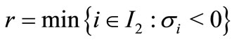 , then ar enters the basis; and if
  , then as leaves the basis.
Like Bland’s anti-cycling rule [9], it can be proved that when the smallest index rule is used to solve system (2.1), cycling doesn’t occur.
Now let us consider the parameter technique by which a new basic solution can be obtained from the current table by changing the right-hand side terms of some basic (in) equalities.
For a basis of (2.1), let IB and IN denote the index sets of basic and nonbasic vectors respectively and ![]() be the basic solution. Suppose
be the basic solution. Suppose
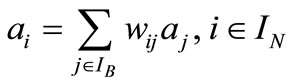 .
.
Multiply both sides by![]() , since aj
, since aj![]() = bj, j Î IB, to have
= bj, j Î IB, to have
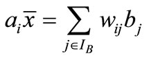 .
.
Therefore the deviation of the nonbasic ai is
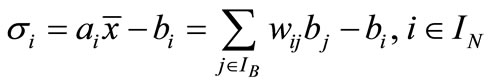 .
.
If bj is changed to bj + dj, j Î IB, the deviation of ai becomes
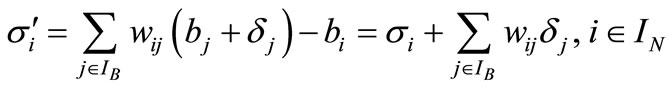 (2.5)
(2.5)
The above operation is denoted by , j Î IB.
Usually we just change the right-hand side of one basic (in) equality such as changing bs to bs + D for an s Î IB. Then the deviation of ai becomes
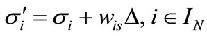 (2.6)
(2.6)
It indicates that when the right-hand side of a basic (in) equality is increased by D, deviations of nonbasic vectors with respect to the new basic solution can be obtained by multiplying the column of this basic (in) equality by D, and then add it to the last column (the deviation column). We will use  to denote such an operation which gives the result (2.6).
3. Convex Quadratic Programming
3.1. Fundamental Concepts and Algorithm
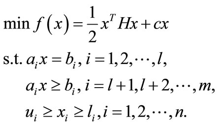
Consider quadratic programming in this form:
 (3.1)
(3.1)
where ,
,  is positive semidefinite,
  ,
,  , bi and li are real numbers.
Let λi be the Lagrange multiplier associated with  or
or , mi be the Lagrange multiplier associated with
 , and ei be the ith row of the identity matrix of order n. The KKT conditions for (3.1) are as follows.
 ,
,
 ,
,
 ,
,
 ,
,
Since
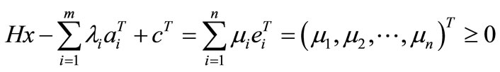 eliminate all the mi from above KKT conditions to have
 (3.2)
(3.2)
We will solve the linear part of (3.2) by Algorithm 2.1 while maintaining all of the complementarity conditions.
(3.2) has n + m variables where λ1, λ2,  , λl are free. In order to initiate the computation, we introduce artificial inequalities

into (3.2). The coefficient vectors of first n + m (in) equalities of (3.2) are
 ,
,
 and the coefficient vectors of last n + m inequalities are denoted by ei which is the ith row of the identity matrix of order n + m, i = 1, 2,
  , n + m.
In system (3.2),
 and
and ,
,
 and
and 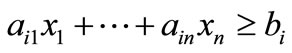
are called complementary inequalities, and their coefficient vectors are called complementary vectors in which
are called Lagrange vectors and
are called constraint vectors, and the associated inequalities are called Lagrange inequalities and constraint (in) equalities respectively.
According to the definition of basic solution of the system of linear inequalities, if one of the complementary inequalities is basic, the corresponding complementarity condition is satisfied. Hence we will keep one of them basic and the other one nonbasic in the computational process.
The initial basic system for solving (3.2) is
 ,
,
 i.e., e1,
  , en, en+1,
  , en+m are initial basic vectors, and

is initial basic solution; hi and ai are initial nonbasic vectors with deviations
 ,
,
 and
and
 ,
,
 .
.
The representation of nonbasic vectors in terms of basic ones and their deviations are given in Table 3.
Since a1,  , al are coefficient vectors of equalities, we first put them into the basis as many as possible. Without loss of generality, suppose that a1,
  , al are

Table 3. Initial table for (3.2).
linearly independent and suppose l pivoting operations can be carried out along the diagonal of the sub-matrix
 .
.
In order to maintain the complementarity conditions, another l pivoting operations are carried out along the diagonal of

which translate the l basic artificial vectors out of the basis. The above 2l pivoting operations are called preprocessing. Since the basic solution must satisfy every equality constraints, once an equality enters the basic system, it is never selected to leave the basic system. For this reason, the columns of basic equalities and the associated rows of artificial inequalities can be deleted from the table. It implies that the upper bound M of the artificial variable may be any number. For convenience of computation, we always take M = 0.
The computational process following the preprocessing is called main iterations where each table is called general (pivoting) table, as shown by Table 4.
Where hN and hB are a partition of the Lagrange vectors , en+N and en+B are a partition of the Lagrange vectors
 , eN and eB as well as aN and aB are partitions of the constraint vectors
  and
and  respectively, and sh, sλ, se, sa in the last column are vectors formed by deviations of the corresponding nonbasic vectors.
We say the principal sub-matrix associated with nonbasic Lagrange vectors and basic constraint vectors to be Lagrange matrix and denote it by L, and say the principal sub-matrix associated with nonbasic constraint vectors and basic Lagrange vectors to be constraint matrix and denote it by G. For the initial table, L = H and G = O; for Table 4,
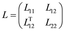 and
and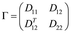 .
.
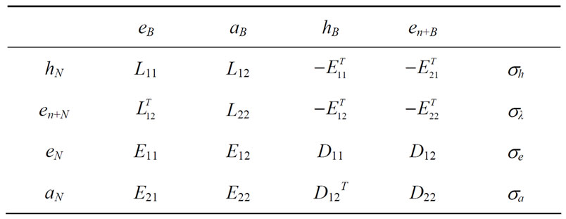
Table 4. The general table.
It can be proved that both Lagrange matrix and constraint matrix are positive semi-definite when the Hessian matrix H of (3.1) is positive semi-definite. A positive semi-definite matrix has the property that if the ith diagonal entry is zero, then all the entries in the ith row and in the ith column are zeros.
Main iterations involve two kinds of operations. One is called principal pivoting which is carried out on a positive diagonal element of the table. The other one is called double pivoting which is carried out on a pair of symmetric off-diagonal elements successively while the diagonal element is zero. The 2l pivoting operations in the preprocessing stage are l double pivoting operations.
The basic solution associated with Table 4 is
 .
.
Besides, we have  and
and . Where lB and lN are vectors formed by the right-hand side terms of basic and nonbasic
 , λB and λN are vectors formed by basic and nonbasic multipliers of λ1, λ2,
  , λm, mB and mN are vectors formed by basic and nonbasic multipliers of μ1, μ2,
  , μn respectively.
Computational steps for the convex QP are as follows.
Algorithm 3.1. Computational steps for (3.2).
Step 1. Initial step.
Let
be the initial basic system and construct initial table given by Table 3.
Step 2. Preprocessing.
For i = 1, 2,  , l, when the deviation of ai is less than, greater than, or equal to 0, go to 1), 2) and 3) respectively.
1) If there is no positive elements in the row of ai that are corresponding to basic inequalities, there is no feasible solution, stop; otherwise carry out a pivoting on one of the positive elements and then carry out a pivoting on the symmetric element.
2) If there is no negative elements in the row of ai that are corresponding to basic inequalities, there is no feasible solution, stop; otherwise carry out a pivoting on one of the negative elements and then carry out a pivoting on the symmetric element.
3) If all the elements in the row of ai that are corresponding to basic inequalities are zero, delete the row of ai and then delete the column of en+i; otherwise carry out a pivoting on one of the nonzero elements and then carry out a pivoting on the symmetric element.
Step 3. Main iterations.
1) If all the deviations of nonbasic vectors (except for nonbasic Lagrange vectors en+1,  , en+l that are corresponding to equality constraints) are non-negative, the current basic solution is the solution to (3.2), stop; otherwise select a nonbasic vector with negative deviation to enter the basis.
2) If there is no positive element in the row of the entering vector that is corresponding to the basic inequality, (3.2) has no solution, stop. Otherwise 3) if the diagonal element in the row of the entering vector is positive, carry out a pivoting on that diagonal element, return to 1); otherwise carry out a pivoting on the largest off-diagonal element in the row of the entering vector, and then carry out a pivoting on the symmetric element, and return to 1).
We will prove that the smallest index rule can prevent cycling even though it may involve more pivoting operations than the smallest deviation rule does. Here each pair of complementary vectors has the same index. For example, hi and ei have index i for i = 1, 2,  , n, and ai and en+i have index n + i for i = 1, 2,
  , m.
, m.
If cycling occurs, some vectors would enter and leave the basis repeatedly. Let s be the largest index of such vectors and consider two tables in the computational process. In one table the sth Lagrange vector enters and the sth constraint vector leaves the basis, and in the other table just reverse. Let P and Q be the principal sub-matrices associated with complementary nonbasic vectors of these two tables, and sP and sQ be deviations associated with P and Q respectively. Then ,
, 
 and
and
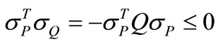
where Q can be partitioned into a 2 ´ 2 matrix as shown in Table 4 or positive definite. It contradicts the assumption that the components of sP and sQ with index s are negative and other components are nonnegative.
3.2. Convex QP with Upper Bounded Variables
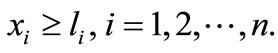
Now let us consider the quadratic programming where variables are bounded from above:
 (3.3)
(3.3)
Let

and let I1 and I2 be a partition of {1,  , n}, i.e., I1 È I2 = {1,
  , n} and I1 Ç I2 = Æ, but empty I1 or I2 is allowed. It can be verified that if
 ![]() is a solution to the system
is a solution to the system
 (3.4)
(3.4)
and every components of ![]() satisfy
satisfy 
 and
and
 , then
 ![]() is the optimal solution for (3.3).
is the optimal solution for (3.3).
The solution of (3.4) is as follows.
Firstly, let I1 = {1, 2,  , n} and I2 = Æ, i.e., ignoring all the upper bounds ui, to solve (3.4) where the first two steps of Algorithm 3.1 are applied. In the following computational process we will make the basic solution satisfy not only
  but also
 . That is we should make deviations of both ei and -ei non-negative. In other words, if the deviation of ei or -ei is negative, then it is a candidate to enter the basis.
If -ei is entering the basis but it does not appear in the table, we change the table as follows. Replace the deviation σi of ei with ui - li - σi, reverse signs of other entries in the row of ei, and then substitute -ei for ei; reverse signs of entries in the column of hi and then substitute -hi for hi. The above operation is called a vector substitution for ei. It amounts to replacing the nonbasic  with
with  and replacing the basic
  with
with . Similarly, if ei is entering the basis but it does not appear in the table, we update the table by conducting a vector substitution for -ei.
Another problem in solving (3.4) is that when a Lagrange vector hi, -hi or en+i is entering the basis, all the entries in this row are non-positive. In this situation, the change of the table is stated in the following 1) and 2).
1) Suppose that the Lagrange vector hi is entering the basis but all the entries in this row are non-positive. In this case we conduct a vector substitution for hi, i.e., reverse signs of all the entries in the row of hi and then substitute -hi for hi; reverse signs of entries in the column of ei and then substitute -ei for ei. It amounts to replacing the nonbasic  with
with  and replacing the basic
  with
with . The associated equalities of the last two inequalities are
  and
and , therefore the change of the right-hand side of
  is ui - li. Considering signs of all the entries in the column of -ei had been reversed, by (2.6) we multiply the column of -ei by li - ui, and then add it to the deviation column. Similarly, if -hi is entering the basis but all the entries in this row are non-positive, we conduct a vector substitution for -hi
2) Suppose that the Lagrange vector en+i (i = l + 1,  , m) is entering the basis but all the entries in this row are non-positive. We see that en+i is a n + m dimensional unit vector with 1 at the (n + i) th position, hi and -hi are n + m dimensional vector whose last m components are not all zeros, and the last m components of constraint vectors are zeros. It implies that the expression of en+i in terms of basic vectors must contain hj or -hj. Suppose that wij is a negative off-diagonal entry in the row of en+i and in the column of
  (= hj or -hj). We conduct a vector substitution for en+i in this way: reverse signs of entries in the column of
  and then substitute
  for
for ; replace the deviation sj of
  (= ej or -ej) with uj - lj - sj, reverse signs of other entries in the row of
 , and then substitute
  for
for . This substitution transforms wij into a positive number so that a regular pivoting en+i ↔
  can be carried out.
Now let us give the algorithm for solving (3.3). In this algorithm, the non-basic vectors include not only those listed in the table but also those that are not listed in the table where  = ei or -ei and
  = hi or -hi.
Algorithm 3.2. Computational steps for (3.4).
Step 1. Initial step, see step 1 of Algorithm.3.1.
Step 2. Preprocessing, see step 2 of Algorithm 3.1.
Step 3. Main iterations.
1) If all the deviations of non-basic vectors except for en+1,  , en+l are non-negative, the current basic solution is optimal for (3.3), stop. Otherwise
2) select a non-basic vector with negative deviation to enter the basis. If the entering vector is ai,  ,
,  or en+i, go to a), b), c), d) respectively.
a) If all the entries in the row of ai that are corresponding to basic inequalities are non-positive, (3.3) has no feasible solution, stop. If the diagonal entry in the row of ai is positive, carry out a pivoting on that entry, return to 1); otherwise carry out a pivoting on the largest entry in the row of ai and then carry out a pivoting on the symmetric entry, return to 1).
b) If  is not listed in the table, conduct a vector substitution for
 . In the row of the entering vector ei¢, if all the entries that are corresponding to basic inequalities are non-positive, (3.3) has no feasible solution, stop; otherwise if the diagonal entry is positive, carry out a pivoting on that entry, return to 1); otherwise carry out a pivoting on the largest entry and then carry out a pivoting on the symmetric entry, return to 1).
c) If the diagonal entry in the row of  is positive, carry out a pivoting on that entry, return to 1); otherwise if there is a positive entry in the row of
 , carry out a pivoting on the largest entry and then carry out a pivoting on the symmetric entry, return to 1); otherwise conduct a vector substitution for
 , return to 1).
d) If the diagonal entry in the row of en+i is positive, carry out a pivoting on that entry, return to 1); otherwise if there is a positive entry in the row of en+i, carry out a pivoting on the largest entry and then carry out a pivoting on the symmetric entry, return to 1); otherwise conduct a vector substitution for en+i, return to 1).
4. Mean-Variance Portfolio Optimization
4.1. Markowitz’s Portfolio Selection Model
Suppose that there are n assets for selection. The rates of return of these n assets are R1,  , Rn (random variables) whose means are r1,
  , rn respectively and the covariance matrix is
  where
where . Let x1, x2,
  , xn be fractions of n assets. The problem is to determine the portfolio (x1, x2,
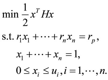
  , xn) so that it has a minimal variance risk at a certain level of expected return rate. It is formulated as follows.
 (4.1)
(4.1)
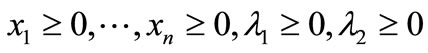
where  and rp is the expected return rate of the investor. Obviously, rp should satisfy
to ensure the feasibility.
The KKT conditions of model (4.1) are
 (4.2)
(4.2)
Add up the n complementarity conditions to have , thus
 .
.
This is another way to compute the variance risk of the portfolio.
(4.1) is a special case of (3.1) mainly in that (4.1) has no general inequality constraints and has feasible solutions. It makes the computation of (4.1) much easy.
Algorithm 4.1. Pivoting algorithm for (4.2).
Step 1. Initial step.
Let
be the initial basic system to construct initial table as shown by Table 5.
Where e1,  , en, en+1, en+2 are coefficient vectors of the initial basic system which are the n + 2 rows of the
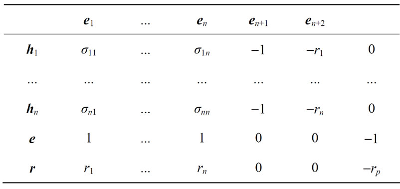
Table 5. Initial table.
identity matrix of order n + 2, 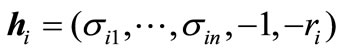 ,
,  and
and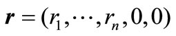 .
.
Step 2. Preprocessing.
Suppose that ,
,  and
and . Carry out four pivoting operations as follows:
e ↔ e1, h1↔ en+1, r ↔ e2, h2 ↔ en+2.
Step 3. Main iterations.
1) If all the deviations of nonbasic vectors except for en+1 and en+2 are nonnegative, the current basic solution is the solution of (4.2), stop. Otherwise
2) select a nonbasic vector (except for en+1 and en+2) with the most negative deviation to enter the basis. If the diagonal entry in the row of entering vector is positive, carry out a pivoting on that entry, return to 1); otherwise carry out two pivoting operations first on the largest entry in the entering vector row and then carry out a pivoting on the symmetric entry, return to 1).
Denote rank (H) by the rank of H. It can be proved that among n basic vectors e1,  , en at most rank (H) + 2 ones may be pivoted out of the basis. It implies that at most rank (H) + 2 components of
  may be nonzeros.
Let ri1,  , riT be the realization of Ri in T periods, then
 . Let
. Let
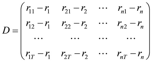 then the covariance matrix
 . Since D is an T ´ n matrix, rank (H) is no more than T. Therefore each portfolio obtained by Algorithm 4.1 contains no more than T + 2 assets no matter how larger n is.
An experiment was conducted by using algorithm 4.1 combining with the parameter formula (2.6) for 70 weekend closed prices of 1072 stocks. Here n = 1072 and T = 70 - 1 = 69. It experiences about 80 pivoting operations to obtain one efficient portfolio and 314 pivoting operations to obtain 20 minimal variance portfolios with different values of rp which are evenly ranging from the minimal mean to the maximal mean of the 1072 stocks. Each pivoting requires about 1074 ´ 1075 multiplications and additions. Therefore the total amounts of computation are 80 ´ 1074 ´ 1075 and 314 ´ 1074 ´ 1075 multiplications and additions respectively. We know that it requires about 10723/3 multiplications and additions to solve a system of 1072 linear equations in 1072 variables by Gaussian elimination.
Now let us give a small example to show how to solve the portfolio problem by using Algorithm 4.1 and the parameter technique introduced in section 2.
Example 1. An investor is interested in three assets. The means of these three assets are 0.05, 0.11 and 0.08and the covariance matrix is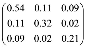 . Solve a portfolio with the minimal variance risk at expected return rate rp = 0.07, 0.08, 0.09 or 0.1.
Solution. The model of this problem is

where , H is the covariance matrix and rp = 0.07, 0.08, 0.09 or 0.1.
The initial table for rp = 0.07 is given by Table 6.
Since the minimal mean is in the first column, we carry out a double pivoting  to have Table 7.
Since the maximal mean is in the second column of the initial table, we carry out a double pivoting ( ,
, to have Table 8" target="_self"> Table 8.
In Table 8, ignoring the deviations of e4 and e5 since they are associated with equalities, there is only one negative deviation -0.2217 taken by h3. Therefore h3 enters the basis. Since the diagonal entry 0.37 in the row of h3 is positive, carry out a principal pivoting on 0.37 to yield Table 9 ignoring the last three columns.
From the column rp = 0.07 we see that all the deviations of nonbasic vectors except for e4 and e5 are positive, therefore the minimal risk portfolio for rp = 0.07 is  = (0.3671, 0.0338, 0.5991), and l1 = 0.4165 and l2 = -3.2117. The variance risk of this portfolio is l1 + l2rp = 0.4165 - 3.2117 ´ 0.07 = 0.1916.
Now consider the portfolio with rp = 0.08. since D = 0.08 – 0.07 = 0.01, by (2.6), we multiply the column of r by 0.01 and then add it and the column of rp = 0.07 to get the column of rp = 0.08. We see that the last three numbers of the column of rp = 0.08 are still positive. Therefore the minimal risk portfolio for rp = 0.08 is  = (0.2095, 0.2095, 0.5811), and l1 = 0.2607 and l2 = -1.4459. The variance risk of this portfolio is l1 + l2rp = 0.2607 - 1.4459 ´ 0.08 = 0.1451.
For rp = 0.09, since D = 0.09 – 0.08 = 0.01, we multiply the column of r by 0.01 and then add it and the column of rp = 0.08 to get the column of rp = 0.09. We see that the last three numbers of the column of rp = 0.09 are positive also. Therefore the minimal risk portfolio for rp = 0.09 is  = (0.0518, 0.3851, 0.5631), and l1 = 0.1050 and l2 = 0.3198. The variance risk is l1 + l2rp = 0.1050 + 0.3198 ´ 0.09 = 0.1338.
In the same way, we can get the column of rp = 0.1. We see that the deviation of e1 is negative and the diagonal entry is positive. Carry out a pivoting e1 ↔ h1 to have Table 10.
From Table 10 we see that the last three deviations are positive. Therefore the minimal risk portfolio for rp = 0.1 is  = (0, 0.6667, 0.3333), and l1 = -0.2811 and l2 = 4.5556. The variance risk of this portfolio is l1 + l2rp = -0.2811 + 4.5556 ´ 0.1 = 0.1744.
4.2. Portfolio of Upper Bounded Assets
For institutional investors some asset such as a stock is not allowed greater than a limited ratio of the total capital. In this situation the model with upper bounded variables is required. Let ui be the upper bound for asset xi that satisfies  and
and  for i = 1,
  , n. This problem is formulated as

Table 6. Initial table for rp = 0.07.
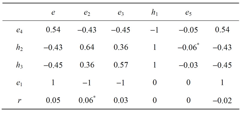
Table 7. Result of first double pivoting.
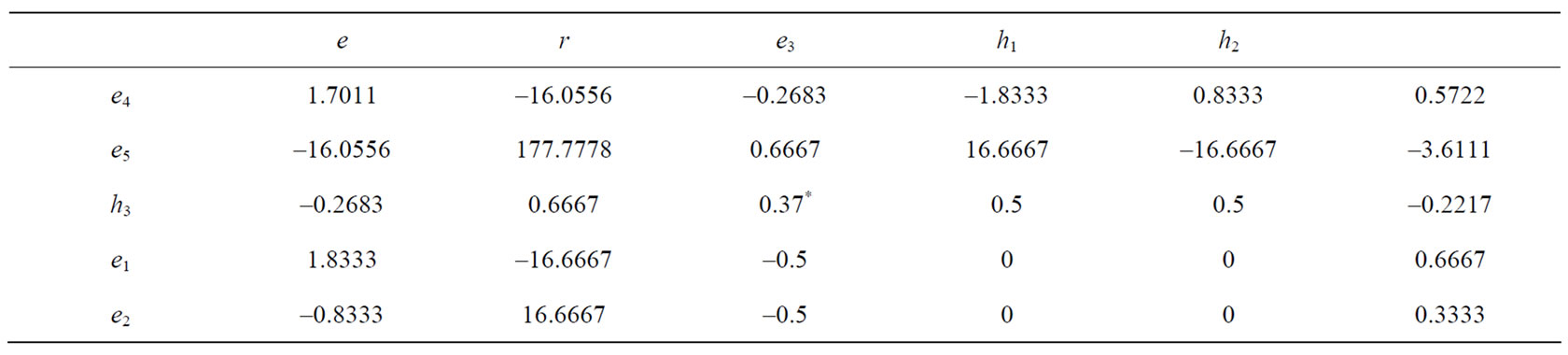
Table 8. Result of second double pivoting.

Table 9. Result of first principal pivoting.
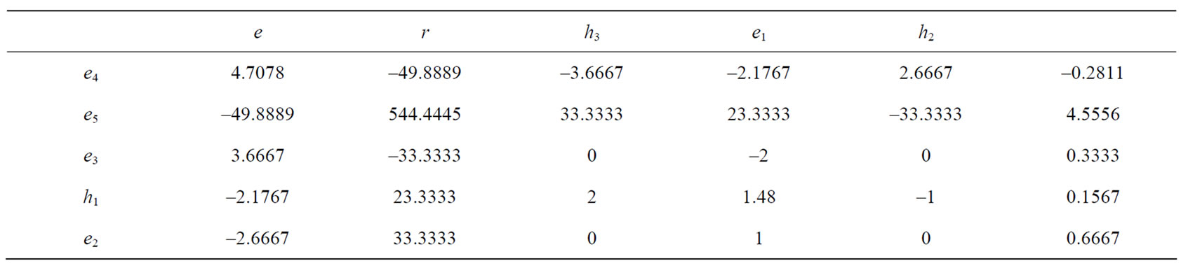
Table 10. Result of principal pivoting for rp = 0.1.
 (4.3)
(4.3)
where  to ensure the feasibility. The minimal value of rp is obtained as follows. Suppose that
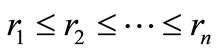 . Distribute 1 to x1, x2,
  , xn sequentially such that
 ,
,  ,
, ,
,  ,
,  where
where  and
and . Then
 .
.
Similarly, we can obtain the maximal value rmax of rp.
The algorithm for (4.3) is as follows.
Algorithm 4.2. Computational steps for (4.3).
Step 1. Initial step, see step 1 of Algorithm 4.1.
Step 2. Preprocessing, see step 2 of Algorithm 4.1.
Step 3. Main iterations.
1) If all the deviations of non-basic vectors except for en+1 and en+2 are non-negative, the current basic solution is optimal for (4.3), stop. Otherwise
2) select a non-basic vector with negative deviation to enter the basis. If this vector is not listed in the table, conduct a vector substitution. If the diagonal entry in that row is positive, carry out a pivoting on that entry, return to 1); otherwise carry out a pivoting on the most positive entry in that row and then carry out a pivoting on the symmetric entry, return to 1).
Example 2. In Example 1, each asset is not allowed to exceed 50%. Solve a minimal risk portfolio with rp = 0.09.
Solution. The initial form is given by Table 11.
As done for Example 1, carrying out 4 pivoting operations e ↔ e1, h1 ↔ e4, r ↔ e2, h2 ↔ e5, and then carrying out a principal pivoting h3 ↔ e3, we have Table 12 where the columns of e and r and the rows of e4 and e5 are deleted.
We see that the third asset 0.5631 is greater than 0.5. Therefore we let -e3 enter the basis. But -e3 is not listed
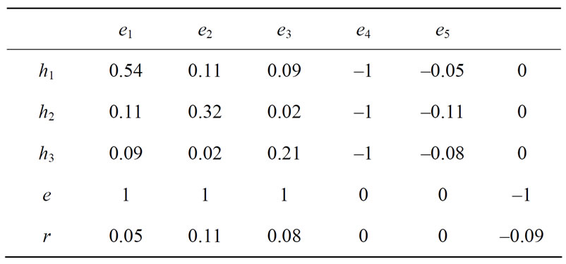
Table 11. Initial table for rp = 0.09.

Table 12. Result of 5 pivoting operations.
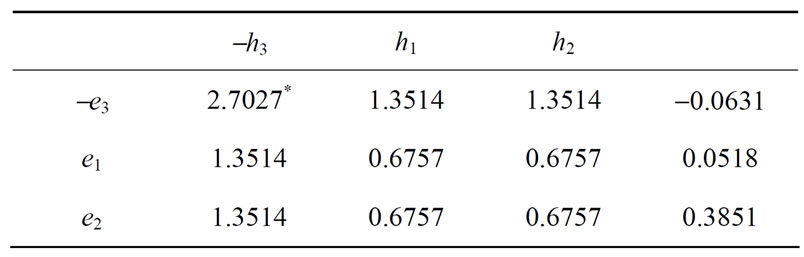
Table 13. Result of vector substitution for e3.
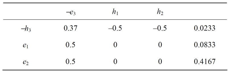
Table 14. Final table.
in the current table. For this we conduct a vector substitution for e3: replace the deviation 0.5631 of e3 with 0.5 - 0.5631 = -0.0631, reverse signs of other entries in the row of e3, and then substitute -e3 for e3; reverse signs of entries in the column of h3 and then substitute -h3 for h3. It results in Table 13.
In Table 13 we carry out a pivoting on the diagonal entry 2.7027 to yield Table 14.
Now all the deviations are positive and no assets are greater than 0.5. Hence we get the required portfolio. Since -e3 is basic, x3 = u3 = 0.5, and x1 = 0.0833, x2 = 0.4167. The variance risk xTHx = 0.1353.
An experiment was conducted by using the same data with n = 1072 and T = 69. For ui = 0.1, i = 1, 2,  , n, it experiences about 95 pivoting operations to obtain one efficient portfolio and 347 pivoting operations to obtain 20 minimal variance portfolios with different values of rp. Each pivoting requires about 1074 ´ 1075 multiplications and additions. Therefore the total amounts of computation are 95 ´ 1074 ´ 1075 and 347 ´ 1074 ´ 1075 multiplications and additions respectively.
5. Conclusions
In this paper we proposed a series of pivoting-based algorithms for solving the following problems:
• the system of linear inequalities;
• convex quadratic programming;
• mean-variance portfolio selection problems.
These algorithms are concise for understanding and efficient for computing as shown by the numerical examples and computer experiments for 1072 stocks. We also proved the convergence of the smallest index rule for convex QP therefore for mean-variance portfolio optimization for the first time.
6. References
[1] R. Fletcher, “Practical Method of Optimization: Constrained Optimization,” John Wiley & Sons, New York, 1981.
[2] J. Nocedal and S. J. Wright, “Numerical Optimization,” Science Press of China, Beijing, 2006.
[3] P. Wolfe, “The Simplex Method for Quadratic Programming,” Econometrica, Vol. 27, No. 10, 1959, pp. 382-398. doi:10.2307/1909468
[4] H. Markowitz, “Portfolio Selection,” The Journal of Finance, Vol. 7, No. 1, 1952, pp. 77-91. doi:10.2307/2975974
[5] H. M. Markowitz and G. P. Todd, “Mean-Variance Analysis in Portfolio Choice and Capital Markets,” Frank J. Fabozzi Associates, Pennsylvania, 2000.
[6] Z. Z. Zhang, “Convex Programming: Pivoting Algorithms for Portfolio Selection and Network Optimization,” Wuhan University Press, Wuhan, 2004.
[7] Z. Z. Zhang, “Quadratic Programming: Algorithms for Nonlinear Programming and Portfolio Selection,” Wuhan University Press, Wuhan, 2006.
[8] Z. Z. Zhang, “An Efficient Method for Solving the Local Minimum of Indefinite Quadratic Programming,” 2007. http://www.numerical.rl.uk/qp/qp.html
[9] V. Chvatal, “Linear Programming,” W. H. Freeman Company, New York, 1983.