Technology and Investment
Vol.2 No.2(2011), Article ID:5164,16 pages DOI:10.4236/ti.2011.22008
A Small-Size Macroeconometric Model for Pakistan Economy
State Bank of Pakistan, Karachi, Pakistan
E-mail: muhammadnadeemhanif@yahoo.com
Received June 25, 2010; revised February 9, 2011; accepted February 15, 2011
Keywords: Macroeconometric Model, Pakistan
Abstract
This paper attempts to develop a small size macro-econometric model for Pakistan to analyze the effects of monetary policy on key macro variables through forecasting and simulations. The model comprises of 17 equations, out of which 11 are behavioral equations while the rest are either identities or definitional equations. OLS method is used to estimate the behavioral equations by using annual data from FY73-FY06. The paper analyzes results of policy simulations to quantify the impact of shocks to various exogenous variables.
1. Introduction
Monetary policy impacts the economy in general and inflation in particular with time lag, therefore, for effective monetary policy implementation, central banks, both in developed and developing countries, are always keen to know the likely effects of monetary policy changes. In the absence of any sound and formal procedure to derive these forecasts, policy makers at central banks have to rely on their own subjective judgments formed on the basis of available information set. Due to its arbitrariness, these judgments often prove wrong to some degree. So, the need arises to have a macroeconometric model to substantiate or form objective judgments on the basis of forecasts generated from the macro model.
The success of dynamic macroeconometric model for US economy spurred the interest of the central banks in developed countries in late 1960s to develop large macroeconomic models for policy making [1,2]. Fair [3,4] also developed macroeconometric models; for the US economy in 1976 and a multi-country model in 1984 for 39 countries. However, the working experience of developed countries about the usefulness of large macroeconometric model in policy making shifted the emphasis from large macroeconometric models to medium and small models. Medium and small size macro models are increasingly developed and used by both developed and developing countries such as England, Australia, Korea, Indonesia, Philippines, China, Malaysia, Kenya, etc. As for Pakistan is concerned, there are few attempts by research organizations and some economists to build large and medium size macroeconometric models such as PIDE Macroeconometric model [5,6]1, Integrated Social Policy Macroeconomic Model [7]2 and Macro econometric modeling and Pakistan’s Economy: A vector autoregression approach [8]3.
But so far, there had been no attempt by State Bank of Pakistan (SBP) to develop a macroeconometric model. This paper is an initial attempt to develop a small size macroeconometric model to have some sort of evaluation process to foresee the effects of monetary policy through forecasting and simulations. This is a small-size model comprising 17 equations, out of which 11 are behavioral equations while the rest are either identities or definitional equations. As the main objective of this model is to foresee the effects of monetary policy through forecasting and simulations, out of fifteen main exogenous variables in the model, seven are directly or indirectly in the control of SBP.
The rest of the paper proceeds as follows. Section 2 outlines the main features of the macroeconometric model, discusses its basic structure, describes inter linkages used in the model and the specification of the behavioral equations. Section 3 presents the data and its sources, discusses estimation approach used to estimate the model, diagnostic tests and forecasting evaluation of the model. Section 4 gives key findings and policy simulations originating from the various monetary and fiscal policy shocks. Section 5 concludes the paper and mentions some limitations of the model and sets out future directions for further extension and development of the macroeconometric model.
2. Basic Structure of the Model4
To model Pakistan’s economy, we have not followed any specific school of thought rather extensively used the economic theory and empirical literature in modeling the macroeconomic variables while ensuring the consistency with the behavior of these variables in Pakistan during 1973-2006. In this model we have eleven (11) endogenous and thirty (30) exogenous variables, where the latter also includes the predetermined (lagged) and dummy variables, as well.
In line with other econometric models, this model also assumes that households make their decisions (about consumption, supply of labor, demand for money, etc.) by solving their maximization problems. Firms mainly take decisions for investment, production, and employment5. Assuming government investment spending to be exogenous we, as such, have not included the other aspects of the fiscal sector. We have also modeled imports and exports of goods and services. In order to analyze the impact of monetary policy on the various macroeconomic variables, behavioral equations of interest rate and consumer price index are used in the model.
Figure 1 presents flow chart of the model which illustrates the relationships between endogenous and exogenous variables. The lists of the equations and identities are reported in Appendix 1. At the bottom part of the flow chart, all non-bold variables are the exogenous variables while all bold variables are either endogenous variables or variables used in the identities. The behavioral equations (shown through shaded blocks), definitional equations and the identities are distinguished with different arrows.
2.1. Behavioral Equations
The model consists of 11 behavioral equations for Consumption, Private Investment, Exports of goods & services, Imports of goods & services, Money Demand, Money Multiplier, Overnight Call Money Rate, Weighted Average Lending Rate, food and non-food Consumer Prices and GDP Deflator. The final specifications of these behavioral equations are discussed below.
2.1.1. Consumption Function
Aggregate consumption is the major component of aggregate demand. At initial development stage of the model, we followed Random Walk consumption function [9]6 and Absolute Income Hypothesis; however, these consumption specifications have been rejected as they have failed to pass a number of diagnostic tests about specification validity. Among competing specifications, the following model of consumption was selected as it relatively better explains the behavior of aggregate consumption over the estimation period for Pakistan economy.
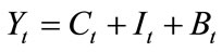
 (1)
(1)
While estimating Ct, Yt and M2 are used in natural log form. Consumption function suggests that current consumption depends (positively) on current income, (negatively upon the) opportunity cost of consumption, (positively upon) M2 (the proxy of financial wealth)7 and adaptive expectations or ratchet effect [10] to captured through lag consumption.
2.1.2. Investment Function
The second major component of aggregate demand is investment which is a key variable for achieving and sustaining higher economic growth. Given the active role of the government not only in providing infrastructure facilities, but also its role in social and economic activities, public sector investment is likely to induce private sector investment. Therefore, in order to incorporate the well established ‘crowding-in phenomena’ in Pakistan [11],8 we have divided the aggregate investment into
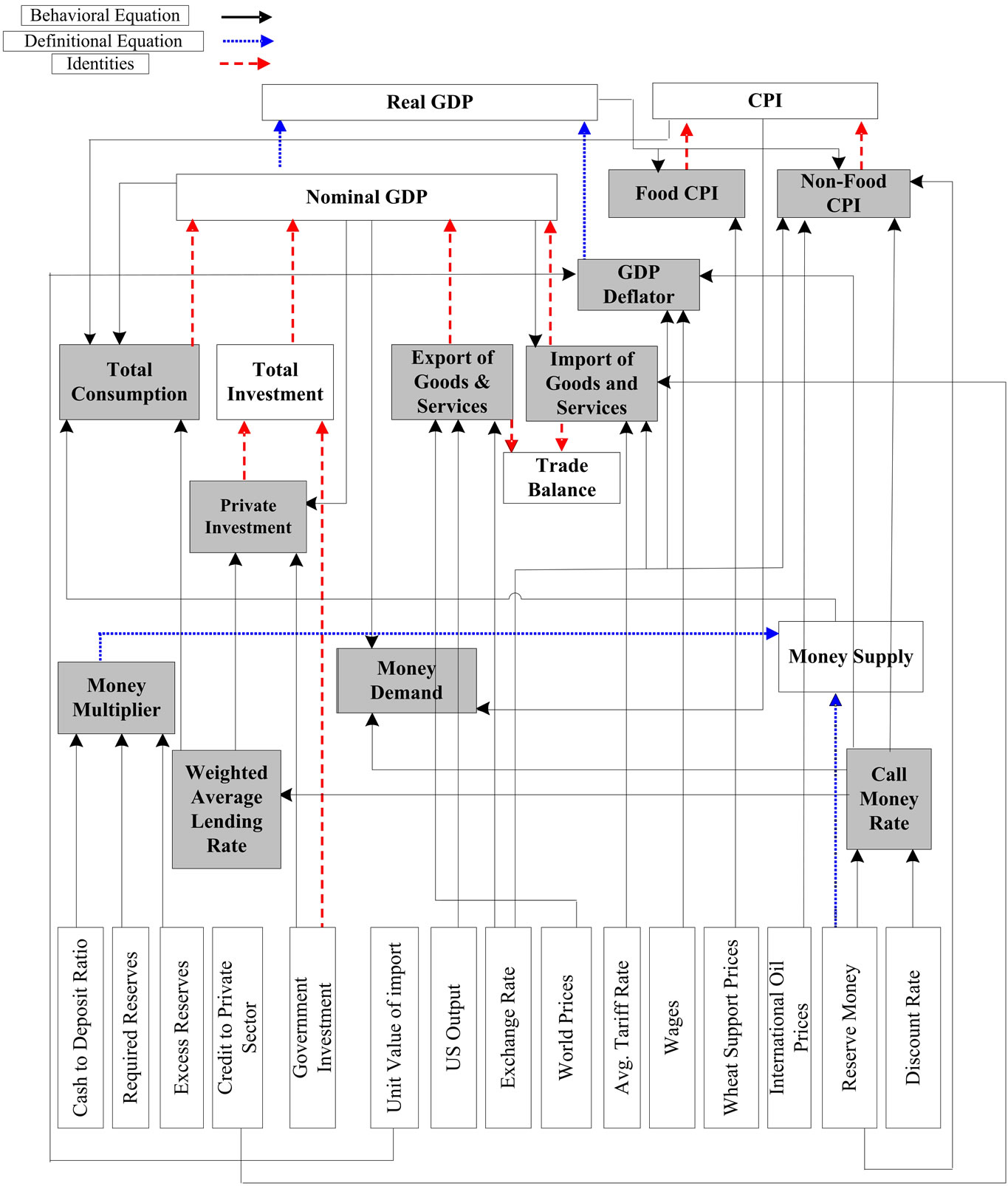
Figure 1. Flow Chart of the model.
private investment and public investment. Since government has the discretion to decide outlay for the public investment, we have treated public investment as an exogenous variable while private investment is modeled as behavioral equation with former as its explanatory variable.
Keeping the Classical and Keynesian investment theories in mind, we have also included interest rate and income. Other explanatory variables such as private sector credit, lags of investment, proxy for uncertainty (either inflation or standard deviation of inflation) are also tested in the private investment equation and, finally, following specification of investment function is selected on the basis of theoretical as well as empirical underpinnings.
 (2)
(2)
All variables except weighted average lending rate are in natural log form. Estimated equation of private investment suggests that nominal GDP with one period lag, level of public sector investment, real interest rate and lagged private investment explained the private sector investment expenditures. We expect the sign of coefficient of real interest rate to be negative. The sign of the coefficient of public sector investment depends upon whether the government investment crowds in or crowds out the private sector investment. On the basis of accelerator model we expect sign of coefficient of the lagged nominal income to positive.
2.1.3. Export of Goods and Services
Export of Goods & Services equation is assumed to depend positively on relative price level in international and domestic markets, foreign demand (represented by foreign income level), and nominal exchange rate. In order to capture the partial adjustment effects, the lagged dependent variable is also included among explanatory variables. Initially, imports of capital goods, total investment, and export refinancing were also included but dropped from the final specification as turn out to be statistically insignificant. All the variables in the following equation are in natural log form except the relative price level.
 (3)
(3)
2.1.4. Import of Goods and Services
Import of Goods & Services is assumed to depend on GDP (as a domestic demand variable represented by income level), exchange rate, credit to the private sector and average tariffs rate. The lagged dependant variable is also included in the equation to capture partial adjustment in imports and to remove autocorrelation. Relative price of imported goods, which is defined as the ratio of the unit value index (import) to the domestic price level, also included in the equation but dropped from the final specification as it turned out to be statistically insignificant.
 (4)
(4)
All variables are taken in logarithmic form except the average tariff rate. Equation (4) describes that the domestic output level and the credit availability positively impact the imports, as with the rise in output level, domestic absorption level will also rise, thus leading to rise in the imports. Similarly, the credit availability would also increase imports (for example of capital goods) by inducing the private investment. The exchange rate and the tariffs will have a negative impact on the imports, as both cause the imports prices (in local currency) to rise and there will be a resultant decline in level of imports.
2.1.5. Money Demand
To model demand for money, we have utilized the traditional money demand function which is determined by the income and the interest rates levels in the economy. Several proxy variables and specifications were analyzed. Specifically, for opportunity cost of money, we used several proxies such as overnight call money rate, weighted average deposits rates, weighted average lending rates and inflation rate. We also bifurcated Log(Yt) into Log(Pt, yt) to discern whether demand for money is more sensitive to the price changes or real income. Given the considerable impact of financial sector liberalization reforms, which were initiated in the beginning of 1990s, on money demand behavior, which renders the (broad) money demand function (MDM2) unstable9, we included a structural dummy in MDM2 equation. In spite of including the structural dummy, the MDM2 remained unstable, which ultimately left no option for us but to rely on narrow money balance (M1) demand function which we found to be stable.
 (5)
(5)
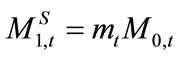
2.1.6. Money Multiplier
Efforts to model money multiplier for narrowly defined monetary balances reveal that the variation in money multiplier is largely explainable by its own lag, excess reserves to M1 ratio, currency to demand deposits ratio, and required cash reserve ratio.10 Parsimonious form selected for money multiplier equation is as follow:
 (6)
(6)
2.1.7. Interest Rates
Two behavioral equations for interest rates, comprising weighted average lending rates and overnight call money rate, are included in the model. The rationale for choosing these interest rates emanates from the fact that former interest rate performed well in modeling private sector investment while latter explained some variation in demand for money and non-food consumer prices equation.
Initially, uncovered interest parity (UIP) approach, which states a direct relationship between domestic and foreign interest rates, was used to model interest rates; however, the result shows that UIP does not hold in case of Pakistan.11 Then Edwards-Khan approach, which is more common in modeling interest rates in developing countries, was used and it was found that12 foreign interest rate and exchanges rate did not significantly explain the domestic interest rates in Pakistan. These results seem plausible given a limited openness of the country, which though increased in the last few years. After estimating several equations, following specifications are found parsimonious for interest rates.
 (7)
(7)
 (8)
(8)
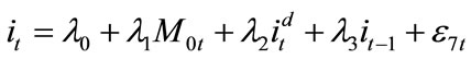
An overnight call money rate is assumed to depend on reserve money, discount rate and lagged dependent variable. Similarly, weighted average lending rate (WALR) is determined by overnight call money rate, lagged weighted average lending rate and a dummy variable (D91) representing a structural break occurred in 1991 due to the change in the methodology of computing weighted average lending rates by SBP.
2.1.8. Prices
Modeling prices is one of the most important components of macroeconometric models used by central banks. In this model, three behavioral equations related to prices are included. First two equations, food and non-food, are related to consumer price while third equation is for GDP deflator, which was required to compute the real GDP from the estimated/forecasted nominal GDP.
Since the monetary policy influence non-food prices more than food prices (which is mainly supply driven), it is desirable to formulate two separate equations one for food group and other for non-food group and then use an identity to have consumer price index which is the weighted average of food and non-food groups.
 (9)
(9)
 (10)
(10)
 (11)
(11)
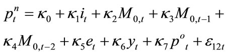
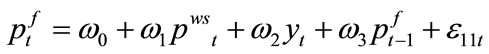
Food-CPI is determined by real GDP and support price of wheat (as specified in Equation (9)) while the Non-food CPI is explained by real, monetary, and the external indicators (as shown in Equation (10)). Given the instability of broad money demand function, M0 and M1 were tested to capture the impact of monetary policy on non-food CPI. We found reserve money to be the most plausible in explaining the variation in prices between these two definitions of money. We have also used overnight money rate in the non-food CPI equation to capture the cost of production impact of changes in interest rate. From supply side, real GDP and international oil prices are included with former representing the availability of goods and services in the economy while the latter reflects the changes in production and transportation cost. Exchange rate pass through effect is captured by including Pak rupee/US dollar exchange rate in non-food prices equation. All the variables are in log form except call money rate. As far as GDP deflator is concerned, it is determined by nominal exchange rate, unit value of import, factors cost (overnight interest rate and wages), and lagged deflator as shown by Equation (11).
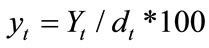
2.2. Identities and Definitional Equation
Four identities and two definitional equations are added to close the models. Among the identities, first is for total investment, which is the sum of Government Investment and Private Investment, where former is treated as an exogenous variable. Second identity represents the trade balance and measure as exports minus import of goods and services (both are endogenous in the model). Third identity is national income accounting identity (nominal GDP), which is the sum of Consumption, Investment and the Trade Balance. Fourth identity is about CPI which is the weighted average of food and non-food CPI while two definitional equations are used in the model for narrow definition of Money Supply (M1) and Real GDP.
3. Estimation of the Model
The sample period used for the model estimation is from FY73 to FY06, covering 34 years. The data is primarily collected from various issues of Economic Survey of Pakistan, and from SBP Publications (see Appendix 2). Given the changes in the base years of the national income account and CPI data, these series are made consistent accordingly at FY00 and FY01 respectively. Before estimation of the specified model, time series properties of each variable were tested through Augmented Dickey-Fuller (ADF) test (for result see Appendix 3).
Ordinary least squares (OLS) method is used to compute individual equations. And those equations recognized to have autocorrelation are corrected by including lagged endogenous variables which has not only solved the autocorrelation problem but also allowed us to incorporate partial adjustment effect. After estimating all the equations, whole set of equations (including identities) are solved simultaneously using the EViews.
While estimating the model, we have used various dummy variables in the individual equations13. The estimated equations of the model are given in Appendix 4 along with the results of the diagnostic tests applied thereon.
3.1. Diagnostic Tests
We evaluate the statistical and theoretical appropriateness of the behavioral equations through various diagnostic tests on residuals. In general, for the estimated parameter to have a statistically desirable property, residuals should be independently and identically distributed (i.i.d.) accompanied by proper specification (which can be checked from Ramsey Reset Test) and normality of residuals is needed for application of most of the testing of hypotheses.
Specifically, we have used the following tests:
• LM test accompanied by the correlogram of residuals and related Q-stat values used for the detection of serial correlation in the residuals;
• Augmented Dickey Fuller test is used to check the assumption of unit root in the residuals of the estimated equation.
• Constancy of residual variance over the estimation period was checked by performing White Heteroscedasticity test and inspecting the correlogram of squared residuals.
• The normality condition of residuals was tested through Jarque-Bera test.
• Structural break in each equation was tested through Chow-Break point test.14
• In addition to theoretical underpinnings and tests on the residuals of each equation, the specification of each equation was also checked by performing Ramsey RESET test15.
• Adjusted R2 and standard errors are also used to evaluate the statistical appropriateness of each equation.
In what follows, these diagnostic tests are explained for estimated private consumption equation for illustration purpose. As exhibited by Table 1, Ljung-Box Q-stat for and LM test are not significant at the 5 percent significance level, suggesting no serial correlation in the residuals, ARCH test and White test which are not significant show that Heteroskedasticity also does not exist in the residuals. From the overall test statistics described above, the residual of the estimated equation appears to be stationary (i.i.d.), which means that the estimated equation is reasonably specified and the statistical appropriateness is adequate. In addition, Jarque-Bera stat is also not significant, suggesting that residuals are normal. Various stability tests, including Chow breakpoint test, suggest that estimated coefficients of the private consumption equation are stable.16
As shown by diagnostic tests in Appendix 4, few estimated behavioral equations related to interest rates and non-food prices fail to pass certain tests17. However, after

Table 1. Diagnostic tests of consumption function.
ensuring that these equations satisfy the alternative stability tests (CUSUM test and CUSUM squared test) we have included these equations in the model due to their importance.
3.2. Forecast Evaluation
Since the main purpose of this model is to analyze the effects of alternative economic policies and to forecast future economic trends, it should have dynamic stability over the complete model besides sound theoretical specifications and statistical appropriateness of individual equations which we have already discussed under the diagnostic tests. In this sub-section, we examine the predictive accuracy of the model through ex post forecast over the sample period to determine how closely the solution values of the individual equations in the model trace the time paths of their actual values.
As exhibited by ex post simulation reported in Table 2, the Mean Absolute Percent Error (MAPE) for both static and dynamic forecasts of most of the behavioral equations lies within the range of 1 to 6 percent (except overnight interest rate) which implies the dynamic stability of the complete model. Further, Theil inequality coefficient of all equations is very close to zero which indicates best fit. More importantly the marginal forecast errors could be traced by inspecting the sum of the two proportion statistics: bias proportion and variance proportion. As shown by Table 2, the sum bias and variance proportions for all equations range between 0 - 5 percent for static forecast accompanied by 0 - 11 percent range for dynamic forecast except money demand and nominal exchange rate equation which have relatively higher bias. This analysis again highlights the strength of the model for forecasting purpose.18
4. Results and Policy Simulations
Appendix 4 gives the detail of estimation results. The key findings of the macro model are the following:
• The government investment has a crowding-in impact on private investment in Pakistan not a crowding-out effect.
• Results suggest that credit channel is more effective in transmitting monetary policy in Pakistan, while the interest rate channel remains weak.
• We have not found any stable specification for nominal money demand function of broad definition (M2), however, demand for narrow money (M1) is found stable.
• US output and exchange rate are the most important determinants of Pakistan’s exports of goods and
• Services while the relative prices are although statistically significant but with a small estimated coefficient.
• Income elasticity of imports is higher than income elasticity of exports in Pakistan which indicates that imports increase higher relative to Pakistan’s GDP while the Pakistan’s exports will increase less proportionally with the rise in the world output.
• Price elasticity (nominal exchange rate elasticity) of exports of goods and services is 0.59 percent which is relatively weaker than the price elasticity of imports of goods and services (0.62).
Reserve money (as compared to narrow or broad money)
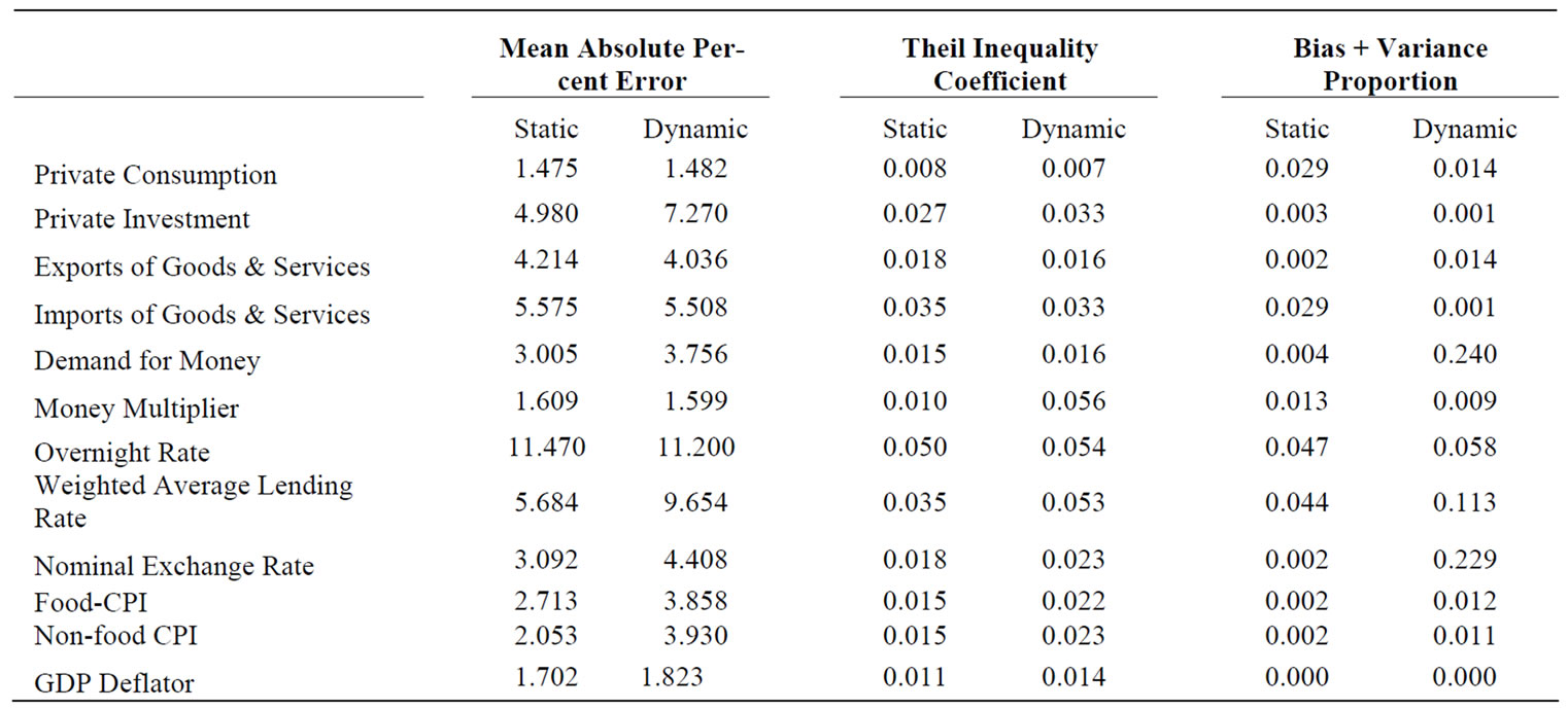
Table 2. Summary statistics for ex-post simulation, FY73-FY06.
has more predictive power in explaining the variation in (non food) prices.
Simulations
Having estimated the model and validated the stability of the model, the next step is to do some medium term policy simulation experiments. Through policy simulation, we can measure the time paths of counterfactual effects of changes in policy instruments or exogenous variables on main macroeconomic variables such as real GDP, private investment, exports and imports of goods and services, prices, etc. Here we consider four shocks comprising both fiscal and monetary policy shocks, i.e., 1) ten percent increase in the government investment for successive two years; 2) one percent reduction in the reserve money; 3) one percent depreciation of the nominal exchange rate; and 4) one percentage point increase in the discount rate for the next two years. Simulation effects are computed using the deviations of major economic variables during one-year ahead and two-year ahead following the aforementioned shocks over the base simulation.
1) Ten Percent Increase in Government Investment When nominal government investment is increased by 10 percent for successive two years, nominal and real GDP grow by 1.48 and 1.37 percentage points respectively above its baseline growth rate during one-year ahead and 0.69 and 0.65 percentage points respectively during two-year ahead (see Table 3). As a result, the CPI inflation will be reduced by 1.01 and 0.15 percentage points respectively for next year and year after. Given the structure of the model, this shock feeds into the endogenous variables through following channels. First, the increase in government investment tends to raise the total investment more as it also lift up the private investment due to crowding in effect of government investment. Second, the rise in the total investment tends to increase the nominal GDP, the effect of higher nominal GDP creeps into CPI, consumption, money demand, imports of goods and services. Specifically, CPI inflation reduced by 1.01 during next year, however, the effect on nominal GDP will dilute in the second year due to the higher interest rate associated with higher money demand. In addition, the higher imports of goods and services associated with higher nominal GDP growth worsen the external account.
2) One Percent reduction in Reserve Money One percent reduction in the reserve money over the baseline for successive two years would directly affect inflation by reducing it by 11 bps and 13 bps during next year and year after over the base line. In addition, as can be seen from Table 3, the reduction in the reserve money would also affect both overnight rate and weighted average lending rate upward, thus, resulting into a slight downward adjustment in the private investment of 0.3 and 0.6 bps during next year and year after. Increase in the interest rate would also reduce the consumption and lead to a slight decrease of 0.2 bps and 0.3 bps in nominal GDP growth and 1 bps each decline in real GDP during one-year ahead and two-year ahead. The decline in the nominal GDP would also reduce the imports of goods and services and would bring some improvement in the external account.
3) One Percent Depreciation in Nominal Exchange Rate One percent depreciation of exchange rate implies an improvement in the competitiveness of exports of goods and services while imports become more expensive, thus, resulting in marked improvement in exports growth by around 63 bps and 43 bps during next year and year after over the baseline growth rate (see Table 3). The increase in exports leads to a gradual improvement in the current account balance. The increase in external demand leads to an upward adjustment in domestic production, the resulting employment generation will increase the household income so as their consumption expenditure. Initially imports declined by 48 bps over the base line growth rate during one period ahead following the adjustment in final demand, but afterwards imports will increase slightly by 0.04 bps during two period ahead, when competitiveness effects begin to dissipate. Thus, the impact on GDP is positive as reflected by the positive deviation of 0.41 bps and 0.30 bps for nominal and real GDP growth respectively from base line growth rate during next period. During two period ahead, positive deviation of nominal and real GDP growth is, to some extent, declined to only 0.26 bps and 0.20 bps respectively. With respect to inflation, the impact of depreciation initially would increase the inflationary pressure through exchange rate pass through to domestic price, however, the effect of higher GDP on CPI would arrest the exchange rate pass through impact and consumer prices declined slightly by 0.02 bps and 0.07 bps during next year and year after respectively19.
4) One Percentage Point Increase in Discount Rate As can be seen from Table 3, if we change the monetary policy stance by raising discount rate by 100 bps, this would first tend to increase the overnight rate which will increase the weighted average lending rate by 20 bps and 59 bps during one-year ahead and two-year ahead respectively. Given the structure of the model, this shock feeds into the endogenous variables through four channels. First, the associated increase in weighted average lending rate raises the user cost of capital inducing a downward adjustment in private investment. Second, the
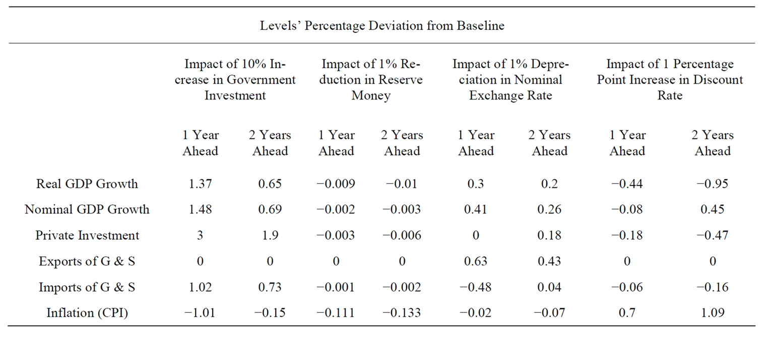
Table 3. Simulation results from various shocks.
increase in interest rates makes saving more attractive for households and induces them to postpone consumption. The downward adjustment in the aggregate demand will reduce the nominal GDP. Third, the reduction in the nominal GDP and the increase in the interest rate would also tend to shrink the money demand as compared to the baseline level. Fourth, as interest rate appears as cost of capital in the equation for non-food CPI and GDP deflator and it has positive sign which would result into higher CPI and higher deflator from these channels. In aggregate, both nominal GDP and real GDP would decline resulting into reduction in the imports of goods and services20 (brining improvement in the trade balance) and hike in the inflation by 0.70 bps and 109 bps during next year and year after over the baseline inflation21.
5. Conclusions and Limitations of the Model
In this paper, we have outlined the basic structure of macroeconometric model for Pakistan and provided the estimation results and policy simulation. As discussed in this paper it is a small-sized model comprising 17 equations, out of which 11 are behavioral equations while rest of the equations are either identities or definitional equations. As the main objective of this model is to foresee the effects of monetary policy through forecasting and simulations, out of fifteen main exogenous variables in the model, seven are directly or indirectly in the control of SBP. OLS method is used to estimate the behavioral equations by using annual data from FY73-FY06. After estimation and applying a set of diagnostic tests, these equations are solved simultaneously using EViews.
The major findings of the model are as follows: 1) the government investment has a crowding-in impact on private investment in Pakistan not a crowding-out effect; 2) results suggest that credit channel is effective in transmitting monetary policy in Pakistan; 3) we have not found any stable specification for nominal money demand function of broad definition (M2), however, demand for narrow money (M1) is found stable; 4) US output and exchange rate are the most important determinants of Pakistan’s exports of goods and services while relative prices are although statistically significant but with a small estimated coefficient; 5) income elasticity of imports is higher than income elasticity of exports in Pakistan which indicates that imports increase higher relative to Pakistan’s GDP while the Pakistan’s exports will increase less proportionally with the rise in the world output; 6) price elasticity (nominal exchange rate elasticity) of exports of goods & services is 0.59 percent which is relatively weaker than the price elasticity of imports of goods & services (0.62); and 7) reserve money (as compared to narrow or broad money) has more predictive power in explaining the variation in price indicators.
Simulation result shows dynamic stability of the complete model as the Mean Absolute Percent Error for both static and dynamic forecasts of most of the behavior equations lies within the range of 1 to 6 percent. Further, Theil inequality coefficient of all equation and two proportion statistics (bias proportion and variance proportion) are very low which indicates very good fit.
Policy simulations experiments were also conducted to quantify the impact of shocks such as: 1) 10 percent increase in the government investment for successive two years; 2) one percent reduction in the reserve money; 3) one percent depreciation of the nominal exchange rate; and 4) one percentage point increase in the discount rate during next year and year after. Simulation effects are computed using the deviations of major economic variables during one-year ahead and two-year ahead following the aforementioned shocks over the base-simulation. Result shows that 10 percent increase in government expenditure tends to raise the total investment more due to crowding-in effect of government investment. Second, the rise in the total investment tends to increase the nominal GDP, the effect of higher nominal GDP creeps into CPI, consumption, money demand, imports of goods and services. One percent reduction in the reserve money, over the baseline during one-year ahead and two-year ahead, tends to reduce inflation by 11 bps and 13 bps more during next year and year after respectively over the base line. This also puts upward pressures on interest rate which in turn results in a slight downward adjustment in the private investment during one period ahead and two-period ahead respectively. The increase in the interest rate would also reduce the consumption and lead to a slight decrease in nominal GDP growth and real GDP growth also bring some improvement in the external account due to reduction in the imports of goods and services. One percentage point upward adjustment in discount rate tends to increase the overnight rate and weighted average lending rates. This would result into lower GDP growth during next year and year after over the base line levels.
This model, in its present form, has following limitations. It is predominantly specified in terms of nominal variables and real GDP growth is computed through relationship between nominal GDP and the GDP deflator. Impact of discount rate appears as a “price puzzle” in this model, although the impact of reserve money on inflation is positive and significant. The model is essentially a demand oriented macro model as the supply side block is not appearing in this model. In addition, fiscal side is only partially captured by incorporating the government investment expenditures as exogenous variables. Furthermore, exchange rate is taken as an exogenous variable in this model which is a very important indicator in an economy. The model captures the long-term relationship but does not shed light on the short term dynamics. This model, nevertheless, can be useful for the policy makers who want to monitor the behavior of core macroeconomic variables and make medium term projections.
6. References
[1] L. R. Klein, “Econometric Fluctuations in the United States,” Wiley, New York, 1950.
[2] L. R. Klein and A. S. Goldberger, “An Econometric Model of the United States, 1929-1952,” North-Holland Publishing, Amsterdam, 1955.
[3] R. C. Fair, “A Model of Macroeconomic Activity,” The Empirical Model, Ballinger Publishing Company, Pensacola, Vol. 2, 1976.
[4] R. C. Fair, “Specification, Estimation, and Analysis of Macroeconometric Models,” Harvard University Press, Cambridge, 1984.
[5] S. N. H. Naqvi, A. H. Khan, N. M. Khilji and A. M. Ahmad, “The PIDE Macroeconometric Model of Pakistan’s Economy,” Pakistan Institute of Development Economics, Karachi, 1983.
[6] S. N. H. Naqvi and A. M. Ahmad, “Preliminary Revised P.I.D.E. Macro-Econometric Model of Pakistan’s Economy,” Pakistan Institute of Development Economics, Karachi, 1986.
[7] H. A. Pasha, M. A. Hasan, A. G. Pasha, Z. H. Ismail, A. Rasheed, M. A. Iqbal, R. Ghaus, A. R. Khan, N. Ahmed, N. Bano and N. Hanif, “Integrated Social Policy and Macro-Economic Planning Model for Pakistan,” Social Policy and Development Centre, Karachi, 1995.
[8] S. Chisti, M. A. Hasan and S. F. Mahmud, “Macroeconometric Modeling and Pakistan’s Economy: A Vector Autoregression Approach,” Journal of Development Economics, Vol. 38, No. 2, 1992, pp. 353-370. doi:10.1016/0304-3878(92)90004-S
[9] R. E. Hall, “Stochastic Implications of the Life Cycle-Permanent Income Hypothesis: Theory and Evidence,” Journal of Political Economy, Vol. 86, No. 6, 1978, pp. 971-987. doi:10.1086/260724
[10] T. M. Brown, “Habit Persistence and Lags in Consumer Behavior,” Econometrica, Vol. 20, No. 3, 1952, pp 355-371. doi:10.2307/1907409
[11] K. Hyder, “Crowding-out Hypothesis in a Vector Error Correction Framework: A Case Study of Pakistan,” Pakistan Development Review, Vol. 41, No. 4, 2001, pp. 633-650.
[12] Cyrus, Sassanpour and Moinuddin, “Experiments with Money Demand Functions for Pakistan,” SBP Bulletin, State Bank of Pakistan, Karachi, 1993.
[13] A. H. Khan, “Financial Liberalization and the Demand for Money in Pakistan,” Pakistan Development Review, Vol. 33, No. 4, 1994, pp. 997-1010.
[14] A. Qayyum, “Modelling the Demand for Money in Pakistan,” Pakistan Development Review, Vol. 44, No. 3, 2005, pp. 233-252.
[15] Moinuddin, “Choice of Monetary Policy Regime: Should SBP Adopt Inflation Targeting,” SBP Working Paper, No. 19, 2007.
[16] S. Edwards and M. Khan, “Interest Rate Determination in Developing Countries—A Conceptual Framework,” IMF Staff Papers, Vol. 32, 1985, pp. 377-403.
[17] S. R. Pindyck and L. D. Rubinfeld, “Econometric Models and Economic Forecasts,” 4th Edition, McGraw-Hill/Irwin, New York, 1997.
[18] M. A. Khan, “Short-Run Effects of Unanticipated Changes in Monetary Policy: Interpreting Macroeconomic Dynamics in Pakistan,” State Bank of Pakistan Working Paper, Vol. 4, No. 1, 2008, pp. 1-30.
[19] C. A. Sims, “Interpreting the Macroeconomic Time Series Facts,” European Economic Review, Vol. 36, No. 5, 1992, pp. 975-1011. doi:10.1016/0014-2921(92)90041-T
Appendix
Appendix 1: Mathematical Representation of the Model
Behavioral Equations
1)  (Consumption)
2)  (Private Investment)
3)  (Exports of G&S)
4)  (Imports of G&S)
5)  (Money Demand)
6)  (Money Multiplier)
7)  (Overnight Call Money Rate)
8)  (Wtd. Avg. Lending Rate)
9)  (Food CPI)
10)  (Non-food CPI)
11)  (GDP Deflator)
Identities & definitional equations
12) 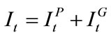 (Total Investment)
13) 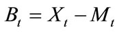 (Trade Balance of G & S)
14)  (Aggregate Demand)
15)  (Consumer Price Index)
16)  (Money Supply)
17)  (Real GDP)
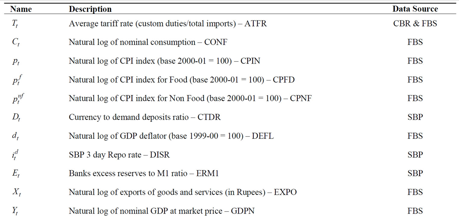
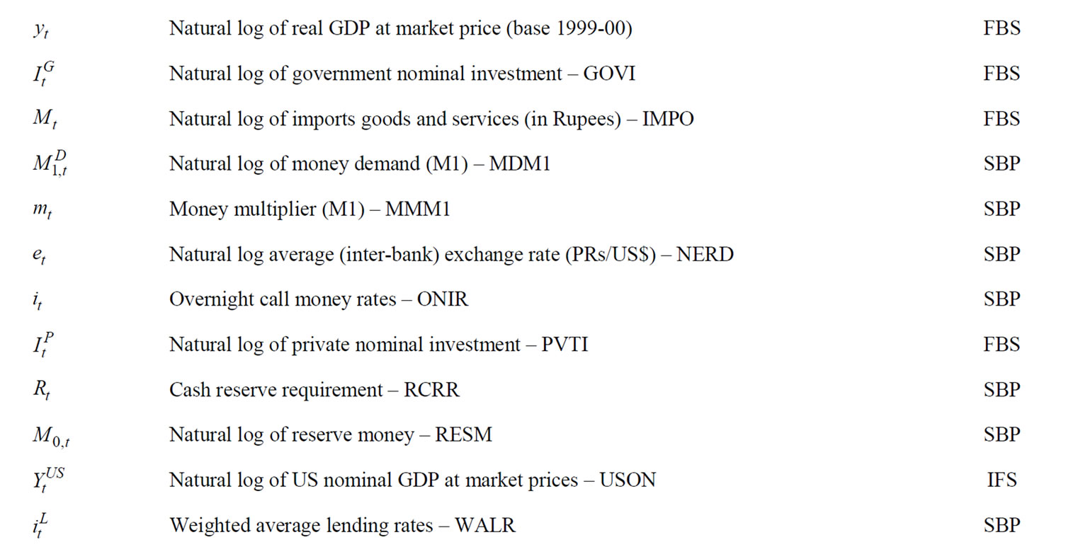
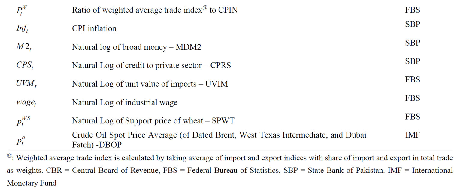
Appendix 2: Variables Description and Data Sources

Appendix 3: Results of ADF test for unit root
Appendix 4: Empirical Result of the Models22
LOG(CONS) = 0.579 + 0.534LOG(GDPN) + 0.263LOG(CONS(−1)) + 0.052DV051 + 0.171LOG(MDM2(−1)) − 0.002(WALR-INF)
Ajd R2 0.999; Std Err: 0.019; DW stat: 1.913; F Test: (0.000);
Ljung-Box Q Stat at lag 10: (0.753); ARCH test: (0.567); LM test: (0.898)
Ramsey Reset Test: (0.266); Jarque-Bera (JB) Test stat: (0.534); Chow Breakpoint Test: (0.326).
LOG(PVTI) = −1.771+ 0.411LOG(GDPN(−1)) + 0.256LOG(GOVI) + 0.425LOG(PVTI(−1)) + 0.067DV04 − 0.008(WALR-INF)
Ajd R2 0.998; Std Err: 0.065; DW stat: 1.987; F Test: (0.000);
Ljung-Box Q Stat at lag 10: (0.682); ARCH test: (0.996); LM test: (0.868)
Ramsey Reset Test: (0.556); Jarque-Bera (JB) Test stat: (0.390); Chow Breakpoint Test: (0.311).
LOG(EXPO) = −0.159 + 0.003WPDP + 0.191LOG(USON) + 0.578LOG(NERD) + 0.687LOG(EXPO(−1)) − 0.200DV821 + 0.142DV911 + 0.044DV04 Ajd R2 0.998; Std Err: 0.066; DW stat: 2.026; F Test: (0.000);
Ljung-Box Q Stat at lag 10: (0.192); ARCH test: (0.632); LM test: (0.762)
Ramsey Reset Test: (0.336); Jarque-Bera (JB) Test stat: (0.082); Chow Breakpoint Test: (0.191).
LOG(IMPO) = −1.544 − 0.011ATFR − 0.624LOG(NERD) + 0.627LOG(GDPN) + 0.279LOG(IMPO(−1)) + 0.318LOG(CPRS−1)) + 0.190DV05 Ajd R2 0.997; Std Err: 0.066; DW stat: 2.130; F Test: (0.000);
Ljung-Box Q Stat at lag 10: (0.802); ARCH test: (0.58); LM test: (0.631)
Ramsey Reset Test: (0.080); Jarque-Bera (JB) Test stat: (0.432); Chow Breakpoint Test: (0.664).
LOG(MDM1) = 1.323 − 0.028ONIR + 0.206LOG(GDPN) + 0.613LOG(MDM1(−1)) + 0.246LOG(CPIN(−1)) + 0.062DV051 Ajd R2 0.999; Std Err: 0.042; DW stat: 1.841; F Test: (0.000);
Ljung-Box Q Stat at lag 10: (0.981); ARCH test: (0.625); LM test: (0.416)
Ramsey Reset Test: (0.131); Jarque-Bera (JB) Test stat: (0.855); Chow Breakpoint Test: (0.288).
MMM1 = 1.915 − 1.741ERM1 − 0.012RCRR − 0.565CTDR + 0.233MMM1(−1) − 0.051DV051 Ajd R2 0.938; Std Err: 0.039; DW stat: 2.149; F Test: (0.000);
Ljung-Box Q Stat at lag 10: (0.935); ARCH test: (0.130); LM test: (0.242)
Ramsey Reset Test: (0.035); Jarque-Bera (JB) Test stat: (0.090).
ONIR = 11.016 − 1.011LOG(RESM) + 0.521DISR + 0.386ONIR(−1) + 2.972DV05 Ajd R2 0.802; Std Err: 1.040; DW stat: 2.300; F Test: (0.000);
Ljung-Box Q Stat at lag 10: (0.987); ARCH test: (0.154); LM test: (0.069)
Ramsey Reset Test: (0.524); Jarque-Bera (JB) Test stat: (0.609); Chow Breakpoint Test: (0.176).
WALR = 1.127 + 0.372ONIR + 0.638WALR(−1)
Ajd R2 0.826; Std Err: 0.857; DW stat: 1.651; F Test: (0.000);
Ljung-Box Q Stat at lag 10: (0.533); ARCH test: (0.923); LM test: (0.484 )
Ramsey Reset Test: (0.743); Jarque-Bera (JB) Test stat: (0.147); Chow Breakpoint Test: (0.003).
LOG(CPFD) = −3.958 − 0.563LOG(GDPR) + 0.576LOG(CPFD(−1)) + 0.210LOG(SPWT) + 0.878LOG(GDPR(−1))
Ajd R2 0.998; Std Err: 0.038; DW stat: 1.421; F Test: (0.000);
Ljung-Box Q Stat at lag 10: (0.391); ARCH test: (0.544); LM test: (0.296)
Ramsey Reset Test: (0.266); Jarque-Bera (JB) Test stat: (0.747); Chow Breakpoint Test: (0.286).
LOG(CPNF) = 6.765 + 0.227LOG(RESM(−1)) + 0.258LOG(RESM(−2)) + 0.196LOG(RESM) + 0.327LOG(NERD) − 0.828LOG(GDPR) + 0.011ONIR + 0.038LOG(DBOP)
Ajd R2 0.998; Std Err: 0.031; DW stat: 1.264; F Test: (0.000);
Ljung-Box Q Stat at lag 10: (0.239); ARCH test: (0.493); LM test: (0.005)
Ramsey Reset Test: (0.005); Jarque-Bera (JB) Test stat: (0.904); Chow Breakpoint Test: (0.001).
LOG(DEFL) = 0.028 + 0.072LOG(NERD) + 0.202LOG(UVIM) + 0.007ONIR + 0.630LOG(DEFL(−1)) + 0.031LOG(WAGE) + 0.045DV04 Ajd R2 0.999; Std Err: 0.021; DW stat: 2.037; F Test: (0.000);
Ljung-Box Q Stat at lag 10: (0.786); ARCH test: (0.236); LM test: (0.816)
Ramsey Reset Test: (0.198); Jarque-Bera (JB) Test stat: (0.305); Chow Breakpoint Test: (0.103).
NOTES
1PIDE Macro Model reflects both the Keynesian and the supply side consideration. It was designed to provide a quantitative framework for an economy wide planning exercise. It comprises four interlinked submodels related to production, expenditure, labor market, foreign trade, and fiscal and monetary sectors. It comprises 97 equations, consisting of 45 behavioral and 52 definitional equations with 86 exogenous variables.
2ISPM, which explicitly recognize the interdependence between macro economy and social sector development, comprises 321 equations out of which 159 are behavioral equations. It can be used as an effective planning tool for social sector development to address poverty and income distribution as well as social service delivery.
3Model [8] comprises ten key macroeconomic variables and was estimated using vector autoregression methodology on Pakistan’s annual data from 1960 to 1988. It empirically analyzes the strength of short-run and long-run impact of anticipated and unanticipated monetary and fiscal policies; and external resources and remittances shocks on the economy.
4It is important to mention that the model in this paper is predominantly in nominal form (like that of one of Bank of England models http://www.bankofengland.co.uk/publications/other/beqm/models00.pdf) keeping in mind that sometimes central banks are also in need of looking at the behavior of nominal variables as some central banks (still) target nominal aggregates like M2.
5The supply side consisting of labour supply and production function is not considered in this model.
6Hall’s [9] consumption function essentially incorporates the rational expectations into Friedman’s Permanent Income Hypothesis.
7We have also tried alternative proxy of financial wealth (M2 plus market capitalization of stock exchange), however, it turns out to be insignificant, perhaps, due to the concentration of capital market in two major cities (namely Karachi and Lahore) and therefore essentially does not explain the aggregate consumption behavior.
8It is important as public sector investment can be used as a fiscal policy tool, and thus using it as separate variable will help in doing the policy simulations and forecasting.
9Literature on money demand for Pakistan documents the mixed results about the stability of the money demand function. Some studies [12,13] find stable money demand function in early 1990s, however, the recent studies [14] done on the most recent data sets find that money demand became unstable due to the implementation of financial sector reforms and financial innovations [15].
10A number of other variables like the difference between the discount rate and overnight call money rate (penal rate) were also tried, but rejected on account of statistical insignificance and/or due to various other diagnostic tests.
11It is pertinent to note that we have not incorporated the country risk factor in the UIP, which is the likely reason to preempt UIP condition to hold. Empirical studies which incorporate the risk factor by using different proxies are generally being criticized on defining the country risk variables and showed mixed trends.
12id = ( * io + (1 − () * ic; where id stands for domestic interest rate, io stands for interest rate in the open economy framework (based on UIP); ic is the interest rate in the ‘closed economy’ framework (subject to domestic policies) and ( = is the weight (between 0 and 1) depending on the ‘openness’ of the economy [16].
13The dummies used are DV821, DV911, DV04 and DV051. DV821 captures the impact of the change in the exchange rate regime from fixed exchange rate to managed float during FY82 in the export of goods & services equation. Similarly, DV911 is included in this equation to capture the post September 11 surge in exports of goods & services. In order to capture the impact of unprecedented behavior during FY05 of the different macroeconomic variables such as private consumption, imports, money demand, and money multiplier, DV051 is used in these particular equations.
14This test in fact splits the sample into two sub samples and compares the statistical differences in estimated equations under null hypothesis of no structural break.
15Ramsey RESET (Regression Specification Error Test) test provides useful information not only for the omitted variables but also about the functional specification of the equation.
16Forecast tests, CUSUM test and CUSUM of squares test are also conducted to ensure the stability of the equation. Forecast test statistics is not significant. In addition CUSUM test stat and CUSUM of squares test stat stay within the 5 percent significance lines throughout the sample period which indicate that coefficients and residual variance are stable.
17These equations fail to satisfy Chow’s breakpoint test which is expected as chow breakpoint test can be only applied on an equation having no dummy variables, therefore, in case of any significant dummy variables, we can not compute the Chow’s breakpoint test.
18For “good” forecast, the bias and variance proportions should be small [17].
19This may seem counter intuitive but this is in response to very small shock to nominal exchange rate of 1%. We may have different result in case the shock is large.
20The reduction in the imports of goods and services, to some extent, will alleviate the downward pressures on GDP.
21The period covered in this study is FY73 to FY06 during most of which SBP has been using reserve money as an operational target rather than discount rate. Thus we found expected impact of changes in monetary aggregates upon inflation. However, positive effect of increase in discount rate upon inflation seems counter intuitive and needs explanation. This phenomenon is well documented in literature for Pakistan [18] and for some other countries [19]. In this model we have used annual data, however, Khan [18] using monthly data from July 1991 to September 2006 found the classic ‘price puzzle’ and explained the positive association between changes in cut-off yields of 6-month T-bills and future inflation in the light of forward looking behaviour of central banks [19]. Another possible explanation for this puzzle can be that during the period of estimation in this paper, discount rate changes were not exercised frequently rendering the variation in discount rate much lower than that of reserve money which explains inflation in this model.
22Figures in parentheses are the probabilities of rejecting null hypothesis. All the variables on RHS of estimated equations have statistically significant estimated coefficient.