ABSTRACT

An electromagnetic wave is a complex of a vortex and a potential processes. This allows us to omit the Lorentz gauge, formulate a mathematically precise theory, and avoid physics discordances. The mechanism of distribution of complex waves in dielectric and electrical conductive environments was described.

1. Introduction

The theory of electrodynamics was formulated in the end of the 19^th century due to work of Maxwell, Lorentz, Heaviside, and Hertz. It allowed inventing modern radio and television communication devices. Nevertheless, there is still the question whether this theory covers entire complex of electromagnetic effects. There definitely is the ground for this question. First of all, modern electrodynamics based on the Maxwell’s equations does not meet completely the main requirements of the field theory, particularly the Helmholtz theorem [1]. The main discordance is the absence of a potential component of magnetic field. It is usually associated with the lack of monopoles. It is believed that this problem will be solved once such objects are found.

It is also known that there are some issues with describing the electromagnetic wave process. These are primary discordances met in the modern theory of electrodynamics.

1) Energy density function of a single-frequency electromagnetic wave changes spontaneously from zero to maximum.

2) The discordance mentioned above is the result of the change in electric and magnetic components occurring in the same phase. Based on the physical conceptions, the independent variables and should be shifted for. However, mathematic conceptions described in the next paragraph do not allow it.

3) Inputting the phase-shifted laws of electrical and magnetic components in the Maxwell’s equations breaks equality. This is the main reason why first two discordances are generally ignored.

4) The previous statement makes us to suppose that expressions in the left-hand side and right-hand side of the equal sign in the Maxwell’s equations refer to one point, and the processes described by these expressions occur at the same time. This approach excludes completely the possibility of diffusion of electromagnetic process in the space and time because the cause and the effect (which are processes presented in the equations) are not separated; hence, the essence of a dynamic process is ignored.

5) In order to eliminate the fourth discordance, they input different arguments in the left and right side of the d’Alembert wave equations (which are derived from the Maxwell’s equations). In other words, the causes and effects are separated spatially and in time. The outputs of the wave equations are written taking into consideration the lag. However, it is not recommended to use these solutions as inputs in initial Maxwell’s equations because the third discordance reveals.

Consequently, the modern theory of electrodynamics has to put up with conceptual discordances, which contradict physical conceptions, in order to satisfy mathematic conceptions.

We offer in this work the theory, which combines vortex and potential electromagnetic processes and allows eliminating of physical discordances while meeting all the mathematic requirements.

The main goal of this research is creating of a consistent theory of the electromagnetic field. We offer to consider both vortex and potential electrodynamic processes when describing an electromagnetic wave. Such an approach allows eliminating of physical discordances. At the same time, arbitrary mathematical limitations as gauges are not applied.

We point out in closing that now there are enough experimental and theoretical facts, which require revising the existing theory of electromagnetic waves. The electroscalar waves, as they are called, were detected in the experiments by C. Monstein, J. P. Wesley [2], K. Meil [3], B. Sacco, A. Tomilin [4]. The theoretical grounds can be found in the works of K. J. van Vlaenderen [5], D. A. Woodside [6], I. A. Arbab, Z. A. Satti [7], D. V. Podgainy, O. A. Zaimidoroga [8].

2. Theoretical Analysis

When expounding the electrodynamics, people usually do the deductive reasoning: a top-down approach. First, they consider well-known phenomena and laws of electromagnetism, and then use them as a basis to derive the Maxwell’s equations, which are assumed to be the peak of the electromagnetic theory. The wave equations are then derived from the Maxwell’s equations. At the same time, the vector potential is introduced. No physical meaning is actually given to it. Its properties are limited by the Lorentz gauge, which does not have any physical explanation.

Let us use the bottom-up strategy now. We write the wave equations for four-dimensional vector potential:

, (1)

, (2)

where and are permittivity and permeability, respectively, and are current and charge densities, respectively.

Note that the arguments of field sources and field characteristics are different in the equations (1) and (2), therefore their solutions are written as lagging potentials.

Let us try to omit the Lorentz gauge and accept the equation that is more general:

, (3)

where is a scalar function, which has the dimension of a magnetic field.

In this case, giving the full description of a magnetic field requires the use of a four-dimensional vector. The magnetic field has potential-vortex nature. Thus, omitting the gauges allows taking into account both the vortex and potential components of the vector. It corresponds to a classical field theory. Let us formulate the Helmholtz theorem [1] for the vector: if the divergence and the curl of the field, which vanishes at infinity, are defined for each point of the certain area, then the vector field can be represented uniquely (up to a vector constant) as the sum of a potential and a solenoidal fields everywhere in this area:

. (4)

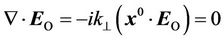
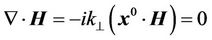
We analyze properties of the vector when the gauge is omitted. Apply the gradient transformation (6) to the well-known equations:

(5)

, (6)

where is an arbitrary scalar time-coordinate function. At the same time, characteristics of a vortex magnetic field, and a vortex electric field, are invariant regarding the transformation (6). Based on this, we conclude that an electromagnetic field is invariant. It is a basis for introducing a gauge. No physical meaning is usually given to the transformation (6).

We will try to explain the physical meaning of this gradient transformation. Note that because of adding to the vector potential its potential component changes. Changing the potential component of a vector field without changing its vortex component is possible when transitioning from a conventionally fixed reference frame К to a steadily moving reference frame. At the same time, it is obvious that the potential component of the electric field should change towards the direction of a reference frame. In the moving (mobile) frame of reference, the electric field of a point charge is not spherically symmetric, but appears as a Heaviside-ellipsoid [9]. In order to compensate this deformation, the negative additive

is input to the Equation (6). However, the deformation of the electric field during transitioning to the moving (mobile) reference frame is taken into account in the equation:

. (7)

The prime symbol here means that calculation of the derivative happens in the moving (mobile) reference frame. In order to describe transformation of the electric field during transitioning from К and (the gradient transformation), it is enough to introduce a curl-free vector potential.

There are two possible types of the vector field transformation: gradient and vortex. The gradient transformation, as it was mentioned before, corresponds to the transition between translational reference frames (one of them can be considered relatively fixed. During the vortex transformation, the transition from a translational (or relatively fixed) frame of reference to a rotating one takes place.

It can be shown rigorously [10] that potential characteristics of an electromagnetic field change during gradient transformation, whereas vortex characteristics are invariant. During vortex transformation, on the contrary, vortex components of an electromagnetic field change and potential ones are invariant. It corresponds to the relative nature of a magnetic field (it depends on a choice of a reference frame) and to its main characteristic, which is vector.

Let us make a conclusion: the ratio of a solenoidal component to a potential component of a vector potential depends on a frame of reference chosen, but this ratio can be defined uniquely in the certain reference frame. The note made in the Helmholtz theorem in brackets shows the relative nature of movement (stability) of any reference frame. If a relatively fixed frame is chosen, it is convenient to set this vector constant to zero. In this case, the indeterminacy in choosing the potentials and disappears, so there is no need to introduce made-up gauges. The theory built up on this basis is called the generalized electrodynamics [10-12].

It is not difficult to derive equations of the generalized geodynamics (the modified Maxwell’s equations) [10-12] from the wave equations (1) and (2) using equations (3) and (5):

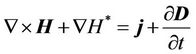, (8)

(9)

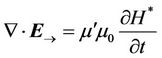
As the result of omitting the Lorentz gauge, the potential (scalar) component of the magnetic field

is kept. We will call it “the scalar magnetic field” (SMF).

Two non-stationary processes

and

are taken into account in the equations of the generalized electrodynamics (8), (9). The first one is called “displacement current”. The second one can be named “displacement charge”. The presence of the “displacement charge” explains the phenomenon of electromagnetic induction, which is confirmed experimentally [10]. The core of this phenomenon is that a potential electric field is induced in the area of a non-stationary SMF. It can be also said that quasi-charges have been appearing.

Two other electrodynamic equations stay the same in the generalized theory:

, (10)

(11)

The equations (8)-(11) and the functions contained in them describe some electromagnetic phenomena. Nevertheless, in order to describe the electrodynamic process fully, it is necessary to use the wave equations (1) and (2) and the main characteristic of an electromagnetic field, which is the four-dimensional vector potential, taking into account its vortex and potential properties.

3. Electromagnetic Waves in Dielectrics

Let us analyze the process of distribution of electromagnetic waves in the fixed (not moving) homogeneous dielectric uncharged environment:

.

The wave equation for the vector splits into two equations for a vortex and a potential component, respectively:

. (12)

. (13)

Let us also write the d’Alembert equations for the vector and the scalar function:

. (14)

. (15)

Thus, an electromagnetic wave has four characteristics. Conventionally, we can distinguish the transverse component of a wave, which is determined by the vortex vectors and, and longitudinal (electroscalar) one, which is characterized by the potential vector and the scalar function.

We can see from the wave equations that velocities of transverse and longitudinal electromagnetic waves are the same. It means that both components of an electromagnetic process are linked indissolubly, and it is impossible to consider them separately in a general case. However, there are some particular cases when differential equations describing these processes are undependable. Moreover, transverse electromagnetic waves, which distribute in the physical (material) environment, generate longitudinal waves at each point, and vice versa.

We assume that some dipole (oscillator) located in the center О creates an electromagnetic wave, which distributes in the dielectric uncharged environment and is analyzed at the long distance from the radiation source. Let us analyze the process close to the point М(x,y), which lays in the coordinate system Oxy. There are both components of the wave at this point: transverse and longitudinal one. Each of them is almost plane, i.e. the distribution front of each wave coincides with the plane, which is perpendicular to the direction of distribution. We assume that the transverse electromagnetic wave distributes along the x-axis and the longitudinal one moves along the yaxis.

We will be guided by physical conceptions when describing the electromagnetic wave process. Within one wave period, four consecutive stages can be distinguished:

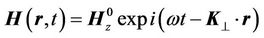
1) generating the vortex magnetic field at the point M(x,y) during the time;

2) generating the vortex electric field at the point M₁(x₁,y₁) during the time;

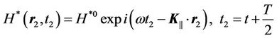
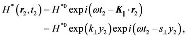
3) generating the SMF at the point M₂(x₂,y₂) during the time;

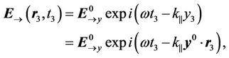
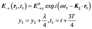
4) generating the potential electric field at the point M₃(x₃,y₃) during the time.

We will suppose that the points M(x,y), M₁(x₁,y₁), M₂(x₂,y₂), and M₃(x₃,y₃) lay consecutively on the line laying in the plane Oxy. Because the velocities of both wave components are the same, the line where these points lay is a bisector of a right angle.

The distance between adjacent points should be taken equal to a quarter of a wavelength. Each next stage occurs with lagging for a quarter of a wave period. Based on the physical conceptions of a wave process, solutions for the differential equations (12)-(15) should be found in the following:

, (16)

(17)

(18)

(19)

here is a circular (angular) frequency. A subscript y or z means the axis where the certain vector is projected. Using (16) in (14) gives us the regular differential equation:

, (20)

Where

is a wavenumber of a transverse electromagnetic wave.

We solve the Equation (20) and get:

(21)

where is an amplitude of a magnitude (strength) of a vortex magnetic field, is a position (radius) vector, which defines the position of the point М(x,y), is a unit vector of the x-axis.

We solve (18) taking into account (23) and get:

(22)

where is an amplitude of a magnitude of a vortex electric field, is a radius vector defining the position of the point M₁(x₁,y₁).

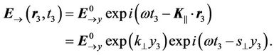
We solve (15) taking into account (18) and get:

(23)

where is an amplitude of a magnitude of a SMF, is a radius vector defining the position of the point M₂(x₂,y₂),

is a wavenumber of a longitudinal electromagnetic wave.

Finally, using (13) and (19) we get:

(24)

where is an amplitude of a magnitude of a potential electric field, is a radius vector defining the position of the point M₃(x₃,y₃).

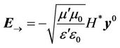
For the vortex electric field:. If we input (22) in this equation, we get:

consequently.

Based on the solution (21), we have the same results for the magnitude vector of the vortex magnetic field:

which means.

Thus, the vortex vectors and are perpendicular to the direction of the wave distribution in case this wave is plane.

Let us input (21) and (22) in the equation (10). As the result of transforming the argument of the vector according to (17) we get:

.

This means that both left and right sides of the equation (10) have the same periodic functions. They cancel each other out, so we get:

.

We can see that the vectors and are perpendicular to each other. This conclusion matches the wellknown conclusion of the conventional electrodynamics.

Let us input the solutions (23) and (24) in (9) when. After transforming the arguments according to (19) we get:

.

In this case, we get the same periodic functions in the left and right sides. Considering this, we have:

. (25)

Consequently, the potential vector is located along the y-axis at any point of the front of a plane wave generated by. This indicates that the term “longitudinal electromagnetic wave” can be used appropriately for the types of the waves studied.

If we input (21) and (22) in (10), and (23) and (24) in (9), we get two equations:

. (26)

As the result, we get the equation of the energy balance between the magnetic and electric components:

(27)

The longitudinal electromagnetic waves transport the energy, as well as transverse waves do. This process is characterized by the vector, which is written like this (in case of plane waves):

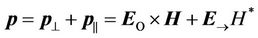. (28)

The direction of the resulting vector coincides with the radius vector drawn from the center О to the point where the field is defined. There are no issues concerning the energy because the function of an electromagnetic energy density looks like this:

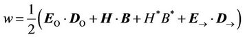. (29)

The first two terms in this formula characterize the energy of a transverse wave, and the two last terms describes a longitudinal wave. If we input the solutions (21)-(24) in (29), then according to the (27) we will get a constant at any time t:

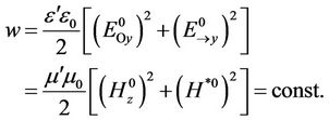(30)

This means that the w function cannot change spontaneously, whereas it happens in the conventional theory. The electric field energy transforms into the magnetic field energy and vice versa. Change of the full energy of an electromagnetic field is only possible because of releasing the heat and transporting the energy according to the well-known law of conversation of energy.

4. Electromagnetic Waves in Electrical Conductive Environment

We will analyze the process of electromagnetic wave distribution in a fixed homogeneous unbounded electrical conductive environment:

.

We rewrite the Equations (8)-(10) like this:

, (31)

, (32)

. (33)

We look for the solutions in the same way as (21)- (24):

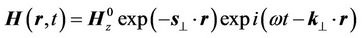
, (34)

(35)

, (36)

, (37)

where

,

are wave vectors, which characterize a complex electromagnetic wave in the electrical conductive environment.

When we input (34)-(37) in the equations (12)-(15), the results are:

(38)

, (39)

. (40)

If we extract and from the equations (39) and (40), and input them in (38), we get the complex equation:

from which we can extract the vortex and potential components easily:

, (41)

. (42)

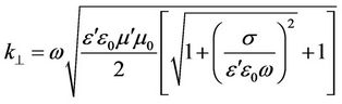
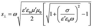
It can be seen that the lengths of the wave vectors in the transverse and longitudinal directions are equal. In a case of an electrical conductive environment, the wave vectors are complex:

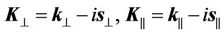, (43)

where

,.

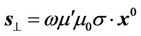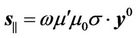If we input (43) in (41) and (41) in (42), we get two biquadratic equations for each type of the waves:

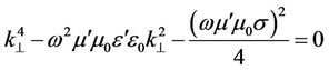, (44)

, (45)

, (46)

. (47)

In the conventional theory, when solving the equations (44) and (45) the real roots corresponding to the physical meaning of the problem are taken into account. The positive real roots correspond to the transverse wave distributing along the x-axis in the positive direction:

, (48)

. (49)

whereas we have the following for the longitudinal electromagnetic waves:

(50)

(51)

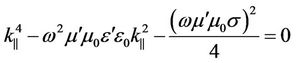
It can be seen that the longitudinal electromagnetic waves damp in the electrical conductive environment. This is also confirmed practically.

As it was mentioned previously, the longitudinal electromagnetic waves have completely different properties, and it should be obviously seen in the theory. The solutions of the equations (46) and (47) have two pairs of roots: two real and two complex (imaginary) ones. When the real roots are chosen, the properties of the longitudinal waves will not differ from the properties of the transverse waves. It does not correspond to the well-known facts. Therefore, we will analyze the case of complex roots. The positive complex roots correspond to the wave distributing along the y-axis in the positive direction:

(52)

. (53)

Taking into account these solutions for the longitudinal electromagnetic wave, which distributes in the electrical conductive environment along the y-axis in the positive direction, gives us:

(54)

(55)

Here, the real values and are used. It should be noted that the values and are equal. Consequently, the amplitude of the longitudinal wave grows in proportion to the damping of the transverse wave. This means that the energy of the transverse wave converts into the energy of the longitudinal wave completely.

For example, such a process takes place in a receiving antenna: due to transverse electromagnetic waves that reach a conductor, a Е-wave is generated in it. Thus, transverse electromagnetic waves damp in an electrical conductor and transmit their energy to a longitudinal wave. A periodic electrical field directed along a conductor generates current impulses.

5. Conclusions

Let us formulate the results of the research in a general way.

The main characteristic of a macroscopic electromagnetic field is a four-dimensional vector. The vector А has both vortex and potential components. A magnetic field is convective change of the four-dimensional vector in a chosen frame of reference. In a general case, a magnetic field is determined by the fourdimensional potential-vortex vector. In any environment, an electromagnetic wave is described by the four wave equations. At the same time, vortex and potential electromagnetic processes are taken into account. Such a theory gives the accurate energy ratios of electric and magnetic components of a field.

The generalized theory of electromagnetic waves provides new opportunities for developing the telecommunication technologies.

REFERENCES

- H. Helmholtz, “Uber Integrale der Hydrodynamischen Gleichungen, Welche den Wirbelbewegungen Entsprechen,” Crelle’s Journal, Vol. 1858, No. 55, 1858, pp. 25- 55.
- C. Monstein and J. P. Wesley, “Observation of Scalar Longitudinal Electrodynamic Waves,” Europhysics Letters, Vol. 59 , No. 4, 2002, pp. 514-520.
- K. Meyl, “Scalar Waves: Theory and Experiments,” Journal of Scientific Exploration, Vol. 15, No. 2, 2001, pp. 199-205.
- B. Sacco and A. Tomilin, “The Study of Electromagnetic Processes in the Experiments of Tesla,” 2013. http://viXra.org/abs/1210.0158
- K. J. van Vlaenderen and A. Waser, “Generalization of Classical Electrodynamics to Admit a Scalar Field and Longitudinal Waves,” Hadronic Journal, Vol. 24, 2001, pp. 609-628.
- D. A. Woodside, “Three-Vector and Scalar Field Identities and Uniqueness Theorems in Euclidean and Minkowski Spaces,” American Journal of Physics, Vol. 77, No. 5, 2009, pp. 438-446.
- A. I. Arbab and Z. A. Satti, “On the Generalized Maxwell Equations and Their Prediction of Electroscalar Wave,” Progress in Physics, Vol. 2, 2009, pp. 8-13.
- D. V. Podgainy and O. A. Zaimidoroga, “Nonrelativistic Theory of Electroscalar Field and Maxwell Electrodynamics,” 2013. http://arxiv.org/pdf/1005.3130.pdf
- E. Purcell, “Electricity and Magnetism,” McGraw-Hill, New York, 1963, 430 pp.
- А. К. Томилин, “Обобщенная электродинамика,” Усть- Каменогорск, ВКГТУ, 2013. http://vev50.narod.ru/Tomilin_ED.pdf
- A. K. Tomilin, “The Fundamentals of Generalized Electrodynamics,” 2013. http://arxiv.org/ftp/arxiv/papers/0807/0807.2172.pdf
- A. K. Tomilin, “The Potential-Vortex Theory of the Electromagnetic Field,” 2013. http://arxiv4.library.cornell.edu/ftp/arxiv/papers/1008/1008.3994.pdf