Journal of Electromagnetic Analysis and Applications
Vol.5 No.8(2013), Article ID:35486,5 pages DOI:10.4236/jemaa.2013.58049
Characteristics of and Control over Resonance in the Electromotive Force of Electromagnetic Induction
![]()
Department of Physics, Chonbuk National University, Jeonju, South Korea.
Email: sbu@chonbuk.ac.kr
Copyright © 2013 Sang Don Bu et al. This is an open access article distributed under the Creative Commons Attribution License, which permits unrestricted use, distribution, and reproduction in any medium, provided the original work is properly cited.
Received April 25th, 2013; revised May 28th, 2013; accepted June 30th, 2013
Keywords: Electromagnetic Induction; Electromotive Force; Resonator, Resonance/Anti-Resonance Frequency
ABSTRACT
The principles of electromagnetic induction are applied in many devices and systems, including induction cookers, transformers and wireless energy transfer; however, few data are available on resonance in the electromotive force (EMF) of electromagnetic induction. We studied electromagnetic induction between two circular coils of wire: one is the source coil and the other is the pickup (or induction) coil. The measured EMF versus frequency graphs reveals the existence of a resonance/anti-resonance in the EMF of electromagnetic induction through free space. We found that it is possible to control the system’s resonance and anti-resonance frequencies. In some devices, a desired resonance or antiresonance frequency is achieved by varying the size of the resonator. Here, by contrast, our experimental results show that the system’s resonance and anti-resonance frequencies can be adjusted by varying the distance between the two coils or the number of turns of the induction coil.
1. Introduction
1.1. Resonance
Resonance occurs widely in nature and is exploited in many man-made devices. Electric resonance is used in many circuits [1-5]; for example, radio and TV sets use resonance circuits to tune in to stations. In these devices, many frequencies reach the circuit simultaneously through the antenna, but significant current flow is induced only by frequencies at or near the circuit’s resonance frequency. By varying the inductance or capacitance, the device can be tuned to different stations. In physics, resonance is the tendency of a system to oscillate at a greater amplitude at the system’s resonance frequencies than at others. At these frequencies, even small periodic driving forces can produce large amplitude vibrations because the system stores the vibrational energy. In this work, we studied electromagnetic induction between two circular coils of wire: one is the source coil and the other is the pickup (or induction) coil, and report the characteristics of and control over the resonance and anti-resonance in the electromotive force (EMF) of electromagnetic induction through free space.
1.2. How Does the Magnitude of Electromotive Force Behave as the Frequency Applied to the Source Coil Increases?
The experiment was performed based on Faraday’s law:
 . (1)
. (1)
where  and
and  are the EMF induced in the induction coil and the magnetic flux passing through the induction coil, respectively [1,6]. The experimental setup consists of two circular coils of wire composed of an electrically conductive copper wire of cross-sectional radius 0.35 mm tightly wound into a series of loops of 5 - 320 turns, radius 7 cm and height 2 cm, as shown in Figure 1. One coil (the source coil) is connected to a signal generator (AFG3021B, Tektronix), and the other (the pickup or induction coil) is connected to an oscilloscope (DSO 5012A, Agilent Technologies). The signal generator supplies a sinusoidal voltage to the source coil, creating a sinusoidal magnetic field. The AC magnetic field propagates through free space and reaches the pickup coil. According to Faraday’s law, an electric field is induced in any region of space in which a magnetic field varies

Figure 1. Schematic diagram of the experimental setup. The experimental setup consists of two coils. Coil A is the source coil, which transmits an electromagnetic wave through free space. Coil B is the pickup (or induction) coil, which detects an induced EMF. Coils A and B are aligned coaxially, such that the distance d between the two coils can be adjusted from 10 mm to 1000 mm. The coils are immobile during operation.
over time. Thus, an EMF is induced in the pickup coil. If the magnetic flux passing through the pickup coil is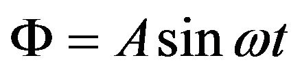 , then the induced EMF is
  . As
. As  increases,
  increases, and the magnitude of
  is proportional to the rate at which the magnetic flux changes with time, so that faster changes give a stronger
 . Here our question is: how does the magnitude of
  behave as
  increases, especially in the high frequency range of 10 kHz to a few MHz?
2. Ease of Use Electromagnetic Induction Properties
2.1. Comparison of the Experimental and Predicted Electromotive Forces
Figures 2(a) and (b) show typical behaviors of 1) the root-mean-square value of 
 of the pickup coil and 2) the phase difference
  between the applied voltage (to the source coil) and the generated
  (in the pickup coil), respectively, as a function of the applied frequency
  (to the source coil). We expected that, according to Faraday’s law and the radiation resistance of the coil,
  would increase with increasing
  and then finally attain a new equilibrium, as shown by the black dashed line in Figure 2(a). Such a response could be modeled using the Langevin function [7],
 . (2)
. (2)
However, the experimental data exhibited a very different behavior, as shown by the red solid circles in Figure 2(a). A resonance behavior was observed at high frequencies, and a relaxation behavior was observed at low frequencies. Resonance and anti-resonance peaks were clearly observed at 87 kHz and 285 kHz, respectively.
Figure 2(b) shows that at a frequency of 10 Hz, the  of the pickup coil was 78˚ out-of-phase with respect to the wave applied to the source coil. As
  increased, the phase difference decreased until the phases matched, where the phase-matching means that the phase difference is less than 5˚. Meanwhile, the phase difference changed profoundly when the pickup coil became resonant. The
  of the pickup coil was 176˚ out-of-phase at frequencies between the resonance and anti-resonance peaks, that is, over a frequency range of 87 - 285 kHz.
The abrupt change in the phase difference may have been due to motions of the charges in the pickup coil. If the phase difference arose from the acceleration of conducting electrons induced by the electromagnetic radiation (generated from the source coil), the phase difference may be effectively independent of  at high frequencies. However, if the phase difference arose from the oscillations in the electric/magnetic dipoles or toroidal dipoles1 [8-14] induced by the electromagnetic radiation, the phase difference would be expected to depend on
  at high frequencies.
The radiation resistance in a coil with  turns composed of an electrically conductive copper wire may be modeled as follows. For a coil of
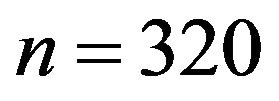 , radius 7 cm and height 2 cm, as used here (see Figure 1), the electric dipole radiation term in the radiation resistance is smaller than the magnetic dipole radiation term, assuming that the distance from the coil is
 , where
  is the speed of light, for example,
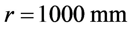 ; the former is on the order of
 , the latter is on the order of
 , where
  and
and  are the angular frequency and the speed of light, respectively. The resonance frequencies obtained in our experiments were much lower than the resonance frequencies of the valence electrons or electric/magnetic dipoles [6,7]. Therefore, in the particular geometry studied here, the abrupt changes in the phase difference may have predominantly arisen from oscillations in the toroidal dipoles [13,14] in the induction coil.
2.2. Adjusting of Resonance and Anti-Resonance Frequencies
To determine whether the resonance frequency  and
and
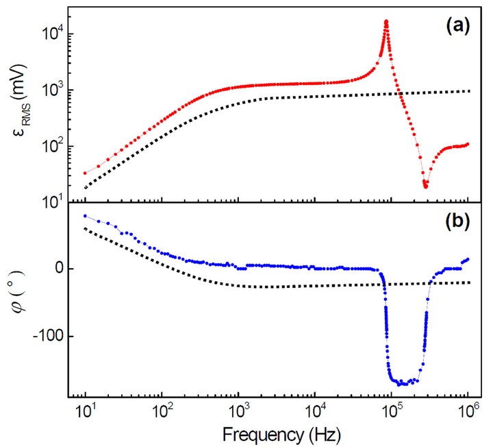
Figure 2. Comparison of the experimental and predicted values of  and
and . The experimental measurements of
  and
and  are shown in (a) and (b), respectively, indicated by red and blue solid circles. The amplitude of the signal applied to the source coil and the distance between the source and induction coils were then fixed at 14 V and 3 cm, respectively. The predicted values of
  and
and  are shown in (a) and (b), respectively, with black dashed lines.
anti-resonance frequency  could be adjusted, we examined the influence of three experimental parameters on the
  and
and . Figures 3(a)-(c) show graphs of
  versus
  for various 1) voltages applied to the source coil (
 = 2, 6, 10 and 14 V), 2) distances between the two coils (d = 10, 30, 100 and 1000 mm), and 3) numbers of turns of the pickup coil (
 = 5, 50, 150, 250 and 320), respectively. Figures 4(a)-(c) show variations of
  and
and  for
for ,
,  and nB, respectively, obtained from Figure 3. The resonance and anti-resonance peaks are clearly evident in most of the curves in Figure 3.
  was not influenced by
  or
or , as shown by the black squares in Figures 4(a)-(b). The interval
  between
  and
and  did not change significantly with increasing
  (Figure 4(a)), whereas
  decreased dramatically as
  increased (Figure 4(b)). These results indicate that
  could be controlled by
  independently of
 . On the other hand, as
  increased,
  and
and  decreased together, as shown in Figure 4(c).
 and
and  each show peculiar behavior. The
  and
and  curves shown in Figure 4(b) indicate that
  does not depend on
  and
and  could be described by an equation involving the logarithm of
 . A plot of
  as a function of
  yielded a straight line, as indicated by the red line in the inset of Figure 4(b). Thus,
  can have the form “
 ”, where
  and
and  are the proportionality constants and the vertical axis intercepts (or meaningless constants), re-
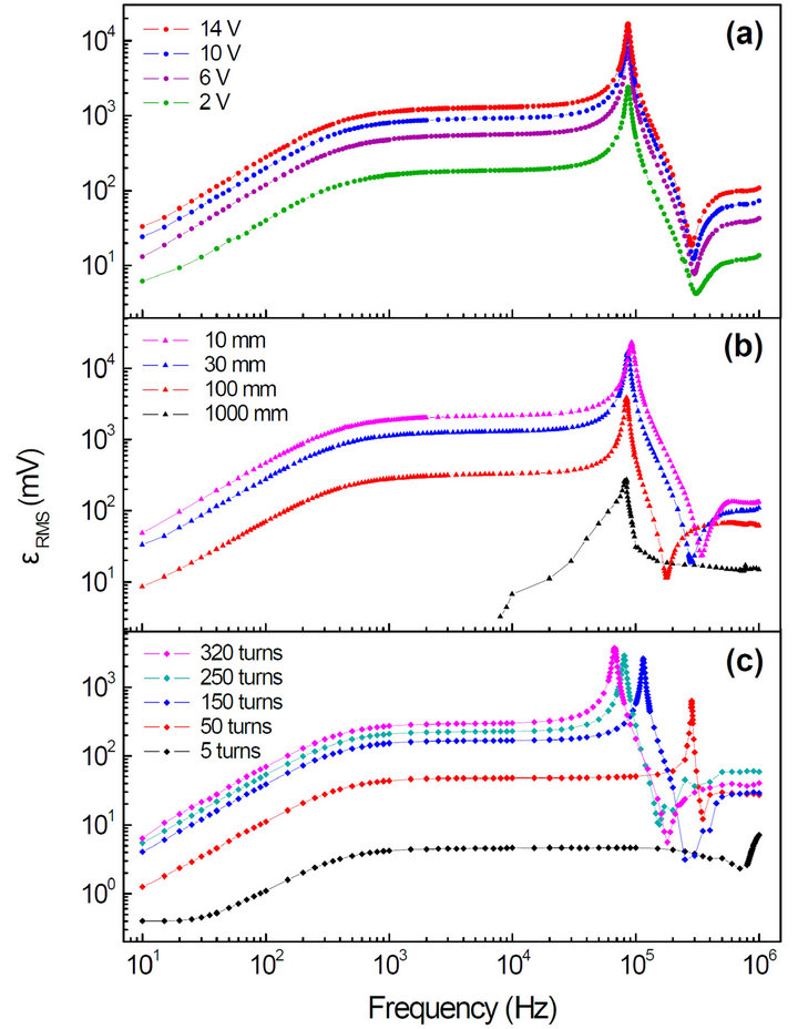
Figure 3. Plots of  versus fA.
  was measured as a function of the voltage applied to the source coil (VA), the distance between the two coils (d) and the number of turns of the pickup coil (nB), where the number of turns of the source coil (nA) was fixed at 320. (a) Plots of
  versus fA for VA of 2, 6, 10 and 14 V, with d and nB fixed at 30 mm and 320, respectively; (b) Plots of
  versus fA for d of 10, 30, 100 and 1000 mm, with VA and nB fixed at 14 V and 320, respectively; (c) Plots of
  versus fA for nB of 5, 50, 150, 250 and 320, with VA and d fixed at 14 V and 100 mm, respectively.
spectively. According to Figure 4(c),  can have the form “
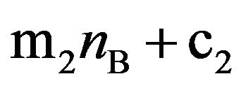 ”, rather than “
 ”, and
  can also have the form “
 ”. The experimental results obtained for various combinations of
 ,
,  and
and  show that
  could be described by an equation of the form “
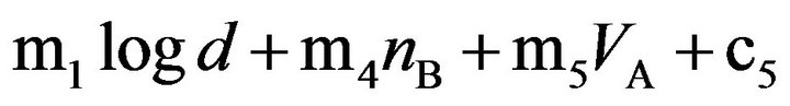 ” with the condition
 , and
, and  could be described by an equation of the form “
 ” with the condition
 . It is noted that under the conditions of various
  turns, all the behaviors of
  and
and  with
with  were like the results shown in Figure 4(b), indicating that the cross term “
 ” might be negligible.
We showed experimentally that pickup coils with different resonance/anti-resonance frequencies could be obtained by selecting the appropriate  and
and  for a given coil size. These results suggest the possibility of “a wireless power transfer station” that transmits power from a source coil to a large number of pickup coils
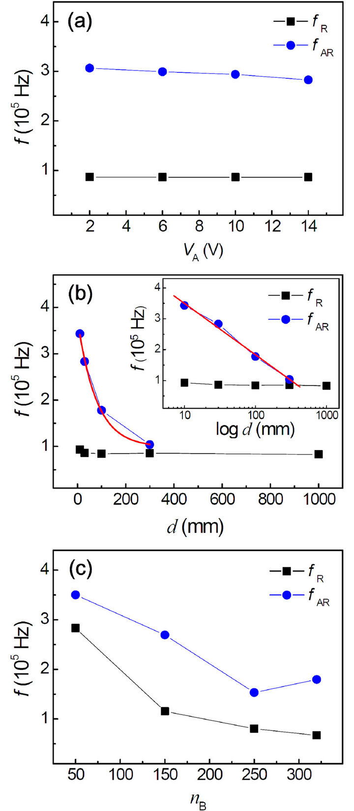
Figure 4. fR and fAR as a function of (a) VA, (b) d and (c) nB.
through free space. If several pickup coils (with different resonance/anti-resonance frequencies) were positioned around a source coil (i.e., a short-range power networking system), power could be transferred from the source coil to the pickup coils by modulating the rate of change (over time) of the magnetic flux passing through each pickup coil. Wireless power transfer stations that are analogous to radio stations may be realized in the near future to permit everyone to use power anywhere without the need for wired power transmission.
3. Conclusion
In summary, we have studied the electromagnetic induction between two circular coils of wire and showed clearly the existence of resonance/anti-resonance in EMF of electromagnetic induction through free space. We believe that our results might provide a competitive approach toward the development of high-efficiency systems in devices of induction cookers, electric power transformers, and wireless energy transfer.
4. Acknowledgements
This research was supported by Basic Science Research Program through the National Research Foundation of Korea (NRF) funded by the Ministry of Education, Science and Technology (grant number 2012R1A1A 2042743).
REFERENCES
- D. C. Giancoli, “Physics: Principles with Applications,” Prentice Hall, Upper Saddle River, 2005, pp. 584-608.
- A. Kurs, A. Karalis, R. Moffatt, J. D. Joannopoulos, P. Fisher and M. Soljacic, “Wireless Power Transfer via Strongly Coupled Magnetic Resonances,” Science, Vol. 317, No. 5834, 2007, pp. 83-86. doi:10.1126/science.1143254
- T. Imura, T. Uchida and Y. Hori, “Flexibility of Contactless Power Transfer using Magnetic Resonance Coupling to Air Gap and Misalignment for EV,” World Electric Vehicle Journal, Vol. 3, 2009, pp. 1-10.
- S. A. Hackworth, X. Liu, C. Li and M. Sun, “Wireless Solar Energy to Homes: A Magnetic Resonance Approach,” International Journal of Innovations in Energy Systems and Power, Vol. 5, No. 1, 2010, pp. 40-44.
- B. Wang, T. Nishino and K. H. Teo, “Wireless Power Transmission Efficiency Enhancement with Metamaterials,” Proceedings of Wireless Information Technology and Systems of 2010 IEEE International Conference, Honolulu, 28 August-3 September 2010, pp. 1-4. doi:10.1109/ICWITS.2010.5612284
- J. D. Jackson, “Classical Electrodynamics,” Wiley, New York, 1999.
- R. Coelho, “Physics of Dielectrics for the Engineer,” Elsevier, New York, 1979, pp. 25-31, 62-73.
- V. M. Dubovik, M. A. Martsenyuk and B. Saha, “Material Equations for Electromagnetism with Toroidal Polarizations,” Physics Review E, Vol. 61, No. 6, 2000, pp. 7087-7097. doi:10.1103/PhysRevE.61.7087
- V. M. Dubovik, B. Saha and J. L. Rubin, “Lorentz Transformation of Toroid Polarization,” Ferroelectrics Letters Section, Vol. 27, No. 1-2, 2000, pp. 1-6. doi:10.1080/07315170008204647
- G. N. Afanasiev, “Simplest Sources of Electromagnetic Fields as a Tool for Testing the Reciprocity-Like Theorems,” Journal of Physics D: Applied Physics, Vol. 34, No. 4, 2001, pp. 539-559. doi:10.1088/0022-3727/34/4/316
- V. M. Dubovik and V. V. Tugushev, “Toroid Moments in Electrodynamics and Solid-State Physics,” Physics Reports, Vol. 187, No. 4, 1990, pp. 145-202. doi:10.1016/0370-1573(90)90042-Z
- K. Marinov, A. D. Boardman, V. A. Fedotov and N. Zheludev, “Toroidal Metamaterial,” New Journal of Physics, Vol. 9, No. 9, 2007, pp. 324-202. doi:10.1088/1367-2630/9/9/324
- A. A. Gorbatsevich and Yu. V. Kopaev, “Toroidal Order in Crystals,” Ferroelectrics, Vol. 161, No. 1, 1994, pp. 321-334. doi:10.1080/00150199408213381
- H. Schmid, “Toroidal Moments in Spin-Ordered Crystals,” Proceedings of One Day International Research Workshop on Super-Toroidal Electrodynamics, University of Southampton, Southampton, 2004, pp. 108-177.
NOTES
1Toroidal moments were first considered by Zel’dovich in 1958. They are fundamental electromagnetic excitations that cannot be represented in terms of the standard multipole expansion. The toroidal dipole moment represents the lowest moment of the third independent electromagnetic multipole family, after the electric and magnetic moments. The properties of materials that possess toroidal moments and the classification of their interaction with external electromagnetic fields are topics of growing interest [8-14].