Journal of Electromagnetic Analysis and Applications
Vol.5 No.10(2013), Article ID:38528,8 pages DOI:10.4236/jemaa.2013.510059
Pulsed Magnetic Field Measurement Outside Finite Length Solenoid: Experimental Results & Mathematical Verification
![]()
1Accelerator & Pulse Power Division, Bhabha Atomic Research Centre, Vishakapatnam, India; 2Electronics & Instrumentation Services Division, Bhabha Atomic Research Centre, Mumbai, India; 3Energetics & Electromagnetics Division, Bhabha Atomic Research Centre, Vishakapatnam, India; 4Accelerator & Pulse Power Division, Bhabha Atomic Research Centre, Mumbai, India.
Email: basushibaji85@gmail.com
Copyright © 2013 Shibaji Basu et al. This is an open access article distributed under the Creative Commons Attribution License, which permits unrestricted use, distribution, and reproduction in any medium, provided the original work is properly cited.
Received March 24th, 2013; revised April 27th, 2013; accepted May 28th, 2013
Keywords: Pulsed Magnetic Field; Biot-Savart Law; Search Coil
ABSTRACT
The paper deals with magnetic field mapping outside a finite length solenoid electromagnet, by an in-house designed and calibrated inductive pick-up or search coil. The search coil is calibrated in a unique methodology based on the azimuthal magnetic field component generated by a straight wire. This unique calibration technique helps us to avoid additional circuitry to integrate the signal obtained from search coil. The methodology proves advantageous in diffusion, implosion studies where the signal frequency changes with dimension and material of experimental job-piece (hollow metal tube). Remedial measures have been taken to avoid electrostatic capacitive pick-up (which eventually exacerbates with integration) keeping measurement simple and accurate. The experimentally measured field values have also been compared with electromagnetic field results obtained from mathematical calculations and finite element based simulations. Two different mathematical approaches have been demonstrated for field computation based on Biot-Savart Law. Both the methods have taken into account the exact geometry of the solenoid, including the inter-turn gaps. The methods use appropriate combination of closed-form mathematical expression and numerical integration techniques and are capable of determining all the vector components of magnetic field anywhere around the finite length solenoid. The mathematical computations are equally significant contributions in the paper especially because exact determination of magnetic fields outside finite length solenoids has not been discussed in sufficient specific details in already existing literature. The mathematical computations, finite element simulations and experimental verification together provide a holistic solution to magnetic field determination problems in pulse power applications that have not been discussed in available literature or books in specific details.
1. Introduction
The magnetic field studies of a finite length solenoid, outside the solenoid, in spite of its importance in many spheres of research and development, are very scarcely researched into. Literature [1-4] concentrates mostly on determination of magnetic field outside an infinitely long solenoid and in some special cases along the axis. Computation of magnetic field around finite solenoid as discussed in [5-8] involves determination of the same by evaluating magnetic vector potential. The present work elucidates two separate computational methodologies involving direct determination of the magnetic field from Biot-Savart law. Pulse magnetic field measurements have been physically carried out and the results obtained have been compared with the computed values.
Pulsed magnetic field measurement is generally performed by inductive principle (i.e. by the help of a search coil [4,9-12]). The literature available however does not describe a method by which the search coil can be calibrated. Novickij [11] has compared the results of the search coil with La0.67Ca0.33MnO3 sensor (employing colossal magneto-resistance principle). The present work attempts to address the problem, executing the calibration in the experimental set up itself, without the requirement of additional integrating circuitry. Electrostatic pick-up signal, which on consequent integration worsens measurement, thus would not be a cause of concern.
The pulsed magnetic field is generated by a finite length solenoid of inductance 14 µH and the measurement is taken just outside the solenoid; the data being important for magneto-forming applications, diffusion studies (interaction of pulsed magnetic field with metallic bodies), applications involving forces generated by coils (e.g. remote displacements of metallic objects where human access is impossible). A standard technique for design of magnetic search coils and a novel method of calibrating it is presented. The results presented in [13] are elaborated and further corroborated with the comparison of the experimental and simulated results with two mathematical computational methodologies.
2. Computational Methodologies for Magnetic Field Estimation
The following sections give a holistic approach towards the computational methodologies involved for field determination. The load coil dimensions are provided in the next section which is necessary inputs for the magnetic field determination of the solenoid coil on being fed with a pulsed current. Since the experiments have been performed in low frequency regime (a few kHz), the spatial current density distribution across the solenoid wire crosssection has been assumed to be uniform.
2.1. Magnetic Field Outside Finite Length Solenoid—Method 1
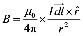
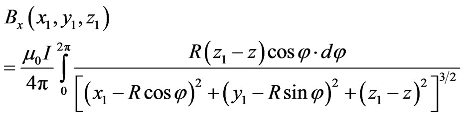
Magnetic field at any point for a current carrying conductor can be calculated by Biot-Savart law as given by the following equation. The computational approach of this method is, dividing the turns of the helical coil into a number of small sections and finding the magnetic field at any point as the vector sum of all the magnetic fields contributed by individual sections.
 (1)
(1)
Here dl is the current element; r is the distance between the current element & the reference point at which the magnetic field is to be measured. Element dl is directed in the direction of current I. A current carrying wire can be divided into a number of elements along its length of same magnitude but of different directions depending on the geometry. The resultant magnetic field at a point will be vector sum of all the magnetic fields due to each current element. Here it is assumed that the wire carries uniform current along its length. This principle of calculation of magnetic field can be utilized to calculate the same for solenoid geometry.
We consider a helical coil of following specifications.
Number of turns : n (21)
Coil inside diameter : Di (55 mm)
Coil length (end-to-end) : lc (87 mm)
Pitch : p (38.5 mm)
(Wire centre-to-centre distance)
Wire diameter : Dw (10 mm)
Now we divide single turn of the coil into N segments along the wire. So each segment sweeps an azimuthal angle.
 (2)
(2)
We define Cartesian co-ordinate system as z axis along the central axis of the helical coil. The x & y axes are along the radial direction but perpendicular to each other. Each current element is having three components dx, dy, dz. The respective current element directions are given by the following equations.
 (3a)
(3a)
 (3b)
(3b)
 (3c)
(3c)
The elemental azimuthal angle is given by the following equation:
 (4)
(4)
Here θ1 & θ2 are the reference angles of the two ends of the current element. Thus for each current element,
 (5)
(5)
The location of each current element or segment is given by:
 (6a)
(6a)
 (6b)
(6b)
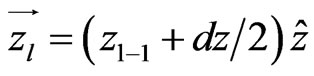 (6c)
(6c)
Here zl−1 is the z co-ordinate of the location of the previous segment. The location of the point at which the magnetic field is to be measured is also given by three co-ordinates is,
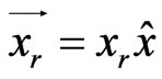 (7a)
(7a)
 (7b)
(7b)
 (7c)
(7c)
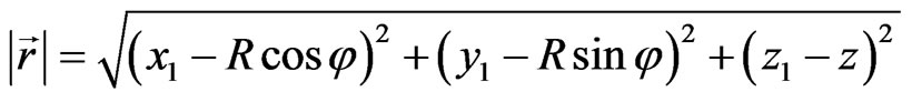
Thus,
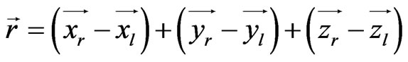 (8)
(8)
Using Equations (5) and (8) in (1) we can find the magnetic field at any given point by a current element.
To find magnetic field at any point by helical coil geometry we have to first initialize the z and θ points. Here zl is started with (Dw/2 + dz/2) and θ1 is started with dθ/2. Finally by integrating the magnetic field at the desired point by each element over all the turns (total n × N elements) we can find the net magnetic field at the point desired by the helical coil. The results of the computational methodology for the present case are given in the later sections.
2.2. Magnetic Field Outside Finite Length Solenoid—Method 2
A method for calculating magnetic field around a solenoid of finite dimensions has already been discussed in the previous section. The present method (Method 2) also determines field around the same solenoid electromagnet using Biot-Savart Law, with certain assumptions. The solenoid electromagnet (which is essentially helical) has been considered to consist of multiple circular current rings of very small cross-sectional area, going around the azimuth of the conductor. The assumption is justified by the fact that, the pitch of the turns in the solenoid is very small compared to the total length of the solenoid and therefore while going around the solenoid, the spatial deviation of current carrying conductor from a plane perpendicular to the axis of the solenoid is not significant. Now that the helical solenoid electromagnet is being represented as a bundle of individual circular current rings going around it, the magnetic field due to the solenoid would essentially be the sum of fields due to each individual current ring. This method specifically takes into account the thickness or depth and width of each turn of the coil, thereby considering the contributions due to its physical dimensions.
Magnetic field generated at any point in the space by a circular current ring, can be determined using the BiotSavart Law, the expression for which is shown in Equation (1). Let us consider a point P(x1, y1, z1) where magnetic field is to be determined due to a current ring which has its centre at O(0, 0, z) and radius as R. Since the ring is circular, position of a current element of length dl on the ring can be represented as (Rcosφ, Rsinφ, z), φ being any angle between 0 and 2π.
For the current element:
 (9a)
(9a)
and,
 (9b)
(9b)
again,
 (9c)
(9c)
Using Equations (9a), (9b), (9c) in Equation (1), magnetic field due to single current ring can be determined at point P as:
 (9d)
(9d)
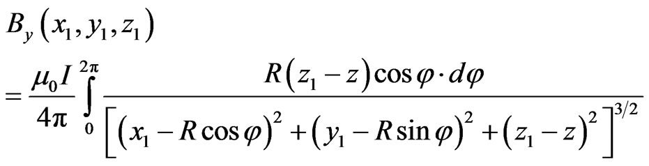 (9e)
(9e)
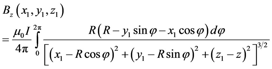 (9f)
(9f)
Equations (9d), (9e) and (9f) represent magnetic fields for a single current ring carrying a current I. In order to determine magnetic field for the solenoid electromagnet, magnetic field generated due to each turn of the conductor were to be summed up. Since the conductor was of finite dimensions, each turn was further divided into a number of circular current rings, fields were determined for each ring, and the contributions from all the rings were finally summed up to obtain total field generated by the solenoid.
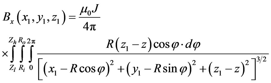
The solenoid coil consists of 21 turns of wire of Assuming that current density J through each turn of the conductor in the solenoid is uniform, expression for magnetic field generated by a single turn of wire having rectangular cross-section, with depth from Ri to Ro and breadth from Zl to Zh, is given as:
 (10a)
(10a)
 (10b)
(10b)
 (10c)
(10c)
The integrals in Equations (10a), (10b), and (10c) were solved numerically. Each single turn of conductor was divided into 625 current rings and field was calculated for each ring and added up to give the magnetic field for corresponding turn of the solenoid. Integral in φ was evaluated from 0 to 2π in 500 steps. Finally, fields due to all the 21 turns were added up to have the field due to total magnetic field at a point due to the solenoid.
2.3. FEM Simulation
The simulation of magnetic field generated by a solenoid was done in FEMM, an open-source computational electromagnetic solver that uses Finite Element Method (FEM) for electromagnetic field simulations [14]. The input to the software are the coil dimensions, number of turns, frequency of operation, peak magnitude of current, boundary conditions. The magnetic field distribution is given in Figures 1 and 2.
The output of the software enables us to determine the magnetic field value at any point in space within the outer boundary for a given current and frequency. Asymptotic boundary condition is used in the outer boundary; mesh was created with 12106 nodes. The centre of the solenoid coil is taken to be z = 0. The position mentioned henceforth is with reference to centre (z > 0 is above the centre, z < 0 is below the centre). The outer boundary dimensions must be much greater than the coil dimensions for proper evaluation of results, a practise being followed in this case.
3. Experimental Setup
The following sections discuss the experimental setup, necessary hardware and procedures adopted for experimentally measuring the pulsed magnetic field.
The components used in the experiments are as follows:
1) 750 µF capacitor bank (15 numbers, 50 µF Yesha make capacitors connected in parallel).
2) Arrangements for charging the capacitor bank.
3) 14 µH solenoid type load coil (21 turns).
4) Spark gap assembly (manual switch).
5) 5 mΩ, 30 W current shunt of T & M Research Products, INC.
6) Search Coil or inductive pick-up coil.
The experimental arrangements are shown in Figures 3-6.
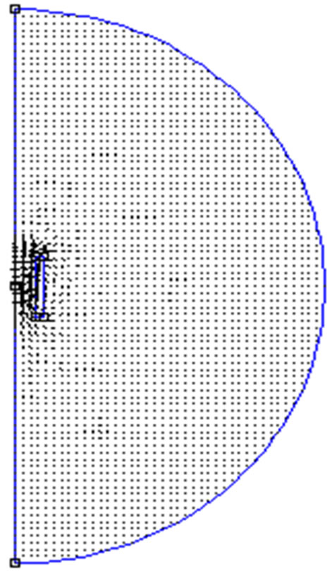
Figure 1. Magnetic field distribution.

Figure 2. Magnified portion of the coil.

Figure 3. Experimental setup.

Figure 4. Schematic of experimental setup.

Figure 5. Radial magnetic field measurement.
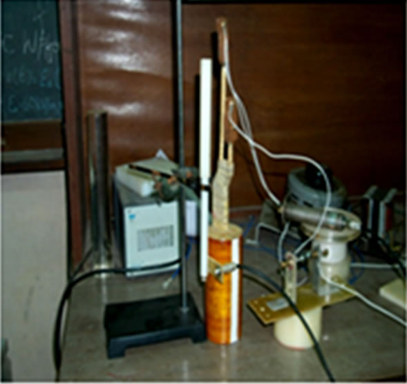
Figure 6. Axial magnetic field measurement.
3.1. Search Coil Design and Calibration
The measurement of pulsed field is based on induction principle [4] and estimation of magnetic field is done based on the induced voltage in the search coil [4,13]. In the present work the search coil has a nylon former, 6 mm diameter, 5 mm length. It was wound with SWG 44 wire, ends being connected to a coaxial connector (supported on FRP sheet). The search coil used in the experiments and its schematic are shown in Figures 7 and 8.
The dimensions are empirical, keeping the small size in mind, but again providing enough space for applying sufficient number of turns to induced measurable voltage in oscilloscope. From the information provided, it can be concluded that the induced voltage in the search coil of N turns by flux linkage of say, “B” T is given as follows (neglecting negative sign).
 (11)
(11)
In the above case, the frequency is 1.389 kHz (the current signal frequency), the cross-sectional area of the search coil is 28.2 sq mm.
Hence for a flux linkage due to 9 mT (the possible field values have been determined by the simulation results discussed in Section 3) and say 60 turns, the induced voltage is an appreciable value of 135 mV well discernable in the oscilloscope resolution. The design was purely mathematical, consistency (field estimation
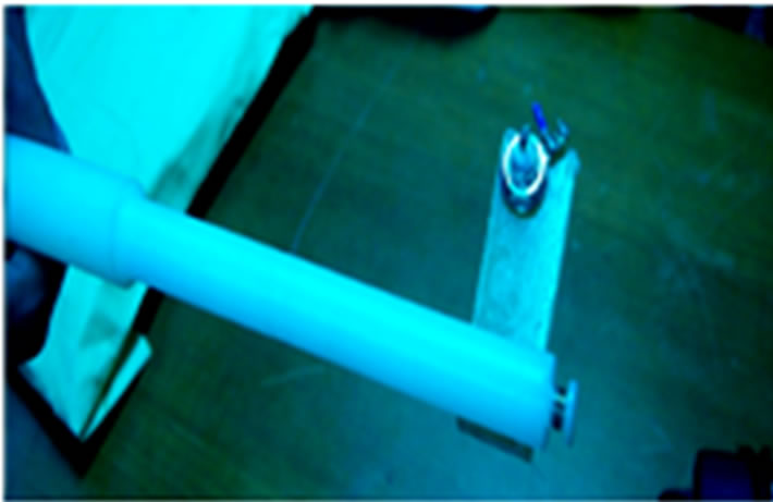
Figure 7. Search coil.
Figure 8. Schematic of search coil.
from induced voltage) of which can only be determined from calibration as in [14]. The experiment has been done by changing the number of turns, before freezing the design for number of turns to be 60. All the results were consistent with the theory. The search coil should be appreciably small in size to closely approximate point measurements and its L/R time constant must be small enough as compared to the rise time of the generating signal to appropriately respond to the same. Both the conditions are met in present case.
The experimental setup for calibration factor (CF) determination [14] is shown below in Figure 9. A relatively long wire is connected between the capacitor bank and the manual switch. The experimental shot is taken by stretching the long wire while keeping the search coil placed directly above the wire. The search coil thus taps the θ-field of the generated magnetic field.
The field generated can be estimated [14: MIT guide] and the corresponding induced voltage recorded in the oscilloscope.
Thus the two parameters, induced voltage and estimated magnetic field is plotted, the slope of the plot gives the value of the calibration factor. The plot is shown in Figure 10.
The waveforms acquired while determining the calibration factor is same as those acquired while measuring the field of the solenoid coil, given later sections. The distance between the wire and the search coil was 1.2 - 1.3 cm, the position dependant parameters,  and
and  are 0.99 and 0.98 respectively.
3.2. Experimental Methodology for Magnetic Field Estimation
The distance between the search coil and load coil centre
Figure 9. Experimental setup of CF determination.
Figure 10. Induced voltage vs. magnetic field: CF is 0.041 T/V.
is 4.83 cm. Keeping this radial distance fixed, both axial and radial magnetic field components are determined by varying the axial distance. The search coil axis must be oriented once in parallel with load coil and another time perpendicular to it for determining the z-field and r-field respectively (Figures 2 and 3 for r and z-field respectively). The pre-charged capacitor bank is discharged in the solenoid load coil through the manual switch to generate pulsed damped current of sinusoid nature; the current in turn generates the field. It should be remembered that the measurement accuracy is position and orientation dependant. The error in the estimation will creep in due to the spatial variation of the search coil, which is unavoidable. It should be kept in mind that the measurement is orientation dependant.
A retort stand and burette clamp was used for holding the search coil firmly in a given position and in proper orientation. These subtle factors were taken care with best possible efforts during measurement.
The current waveform (blue) and the corresponding induced voltage in the search coil (pink or yellow) are shown in the waveforms in the next section. The magnetic field magnitude (radial or axial component) at a given point due a given magnitude of current in the given frequency of operation is given by the product of the peak magnitude of the cosine wave (induced voltage) and the CF (0.041 T/V) determined earlier. The experimental results and validation with each of the computational methods mentioned aforesaid are provided in the sections below.
4. Results & Discussions
In this section we present comparison of magnetic field values obtained through simulations and physical measurements. Axial and radial field values have been discussed with separately.
4.1. Experimental Results: Axial Magnetic Field
The present section deals with the axial magnetic field measurement. Some typical experimental results are shown in the table below. The field measurement is obtained at a fixed radial distance of 4.83 cm from the load coil centre and different axial positions. The typical results depict an axial position near the centre (z = 0.3) and within the coil winding range (z = −2.55) in Figure 11.
The plot of the axial magnetic field values for pulsed peak current of 520 A along the length of the solenoid coil is given in the Figure 12.
4.2. Experimental Results: Radial Magnetic Field
The present section deals with the radial magnetic field measurement. Some typical experimental results are shown in the table below. The field measurement has been obtained at a fixed radial distance of 4.83 cm from the load coil centre and at various different axial positions. The typical results correspond to an axial position near the centre (z = 0.45) and point of maximum radial field i.e. (z = −4.55) in Figure 13.
The plot of the axial magnetic field values for pulsed peak current of 520 A along the length of the solenoid coil is given in the Figure 14.
4.3. Discussion of Results
The aforesaid formulations have been used to solve for magnetic flux density directly and do not involve the intermediate step of determining magnetic vector potential. Although the Biot-Savart method already incorporates computation of magnetic vector potential, therefore the formulations could avoid additional steps of determination of vector potential through direct implementation of Biot-Savart technique.
The formulation of method 1 considers flows of cur-
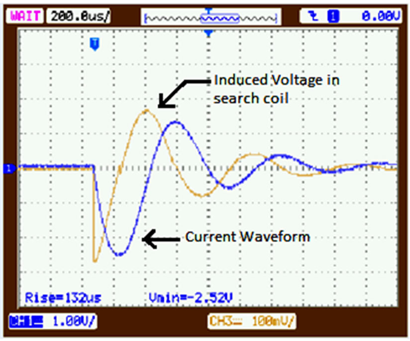
Figure 11. Position(in cm): 0.3, Current (A): 512, Induced Voltage (mV): 272, Bz (simulated in mT): −13.4, Bz (experimental in mT): −11.52, Bz (Method 1 in mT): −11.57, Bz (Method 2 in mT): −13.3, Ch1: 200 A/div, Ch2: 100 mV/div.

Figure 12. Axial magnetic field variation along the coil length.
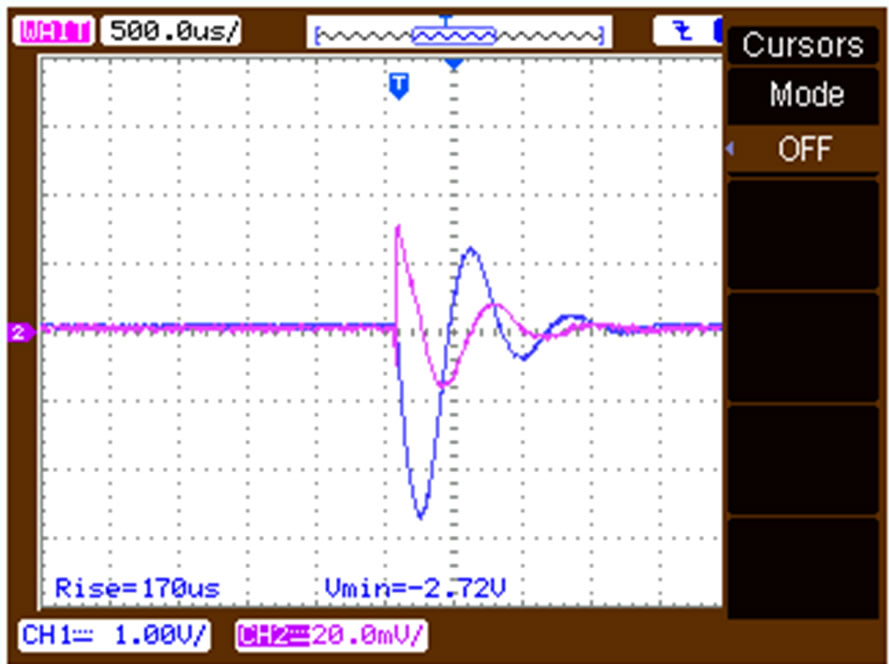
Figure 13. Position (in cm): 0.45, Current (A): 536, Induced Voltage (mV): 31.2, Br (simulated in mT): 1.76, Br (experimental in mT): 1.3, Br (Method 1 in mT): 3.36, Br (Method 2 in mT): 1.8, Ch1: 197 A/div, Ch2: 19.5 mV/div.

Figure 14. Radial magnetic field variation along coil length.
rent through a single representative point on the inner diameter of the load coil, instead of the entire cross-section of the wire. Also, effects of skin depth and proximity effect are not in consideration of the formulation. Hence the results at the edges of the coil show discrepancy with the corresponding FEM simulation results. The formulation in method 2 considers specifically the dimensions of the wire used for winding the coil. Hence it shows better concurrence with the simulated results, than method 1.
The formulation referred as method 2 can also be used to take into account rotational asymmetry in the wire loop and thus has the potential to determine magnetic field for any generic geometry of current carrying loop beyond most idealizations. The concept of current loops is based on the assumption that each turn is basically circular. Therefore it doesn’t consider the ideal helical geometry of the solenoid, although variation in the result would not be significant in the scenario under consideration since the inter-turn distance is quite small. Nevertheless, suitable modifications can always be done in the program to incorporate exact helical geometry of the solenoid. It is being planned for in the next version of the same. The program assumes uniform current density along the solenoid conduct cross-section. While operating in the quasi-static regime, although with the order of frequencies we’ve been dealing with in the current experiment, inaccuracies being introduced from the assumption weren’t significant, yet to be exactly sure of the accuracy of the results being obtained, the next version of the code would incorporate skin effects.
Magnetic field (in theta direction) generated by a straight current carrying conductor has a closed form solution depending only on the position of field probe, with respect to the conductor. Taking precautions for positioning, correlating the field generated with the induced voltage is straight forward at a given frequency. Hence another standard field measuring device, such as Hall probe is not required, thereby establishing its uniqueness. A straight forward calibration factor in V/T can be obtained for a given frequency. The measurement technique is unique in the aspect of employing a differentiated signal in estimating the magnetic field. Thus the usage of extra hardware in terms of RC integrator, amplifier can be safely avoided. However the issue lies in re-calibrating the search coil, every time the frequency of operation changes.
5. Conclusion
The magnetic field generated outside a solenoid coil being excited with pulsed current has been extensively studied and presented in this paper. It is a topic of significant relevance in the field of pulsed power, which is being used in the domain electromagnetic forming. The subtle nuances of mathematical, simulation and experimental results are scarce in available literate, and have been emphasized upon in details in the paper. Numerical formulations of Biot-Savart Law have been used to determine magnetic field around a finite length solenoid. The results obtained theoretically have been compared with results obtained from FEM simulation and experimental results. It is observed that the results obtained through various techniques are in close coincidence with one another. It has also been demonstrated that computational assumptions made during the process can be reasonably accommodated without introducing significant errors in the results. Further refinements in computational and experimental techniques are on to bring down the negligible amount of errors present to even more insignificant levels. The methodology of field determination discussed here can prove to be of great relevance in electromagnetic experiments being carried out on industrial scale.
REFERENCES
- O. Espinosa and V. Slusarenko, “The Magnetic Field of Infinite Solenoid,” American Journal of Physics, Vol. 71, No. 9, 2003, pp. 953-954. http://dx.doi.org/10.1119/1.1571841
- J. Farley and R. H. Price, “Field Just Outside a Long Solenoid,” American Journal of Physics, Vol. 69, No. 7, 2001, p. 751. http://dx.doi.org/10.1119/1.1362694
- B. B. Dasgupta, “Magnetic Field Due to a Solenoid,” American Journal of Physics, Vol. 53, No. 8, 1985, pp. 782-783. http://dx.doi.org/10.1119/1.14318
- H. E. Knoepfel, “Pulsed High Magnetic Fields,” NorthHolland Publishing Company, Amsterdam, London.
- V. Labinac, N. Erceg and D. Kotnik-Karuza, “Magnetic Field of a Cylindrical Coil,” American Journal of Physics, Vol. 74, No. 7, 2006, p. 621.
- A. I. Rusinov, “High Precision Computation of Solenoid Magnetic Fields by Garrett’s Methods,” IEEE Transactions on Magnetics, Vol. 30, No. 4, 1994, pp. 2685-2688. http://dx.doi.org/10.1109/20.305833
- V. I. Danilov and M. Ianovic, “Magnetic Fields of Thick Finite DC Solenoids,” Nuclear Instruments and Methods, Vol. 94, No. 3, 1971, pp. 541-550. http://dx.doi.org/10.1016/0029-554X(71)90019-X
- H. E. Knoepfel, “A Comprehensive Theoretical Treatise for Practical Use,” John Wiley Sons, INC., Hoboken.
- A. S. Bozek and E. J. Strait, “Manufacturing of Magnetic Probe Coils for DIII-D,” General Atomics Report GAA24492.
- P. G. Mattocks, “Copper-Beryllium Search Coils and the Measurement of Small Magnetization Pulsed Magnetic Fields,” Journal of Physics E: Scientific Instruments, Vol. 12, No. 7, 1979, p. 658.
- J. Novickij, R. Kačianauskas and A. Kačeniauskas, “Axial Magnetic Field Measurements of Pulsed,” Elektronika IR Elektrotechnika, 2004. Nr. 2(51).
- S.E. Segre and J.E. Allen, “Magnetic Probes of High Frequency Response,” Journal of Scientific Instruments, Vol. 37, No. 10, 1960, p. 369.
- S. Basu, et al., “Pulsed Magnetic Field Measurement outside Finite Long Solenoid Implementing Novel Calibration Technique,” 7th IEEE International Vacuum Electronics Conference, Bangalore, 21-24 February 2011, pp. 415-416.
- MIT Lecture Notes, Chapter 9, pp. 4-6. http://web.mit.edu/viz/EM/visualizations/coursenotes/modules/guide09.pdf