Journal of Electromagnetic Analysis and Applications
Vol. 3 No. 5 (2011) , Article ID: 5019 , 7 pages DOI:10.4236/jemaa.2011.35022
Nonlinear Oscillations of a Magneto Static Spring-Mass
![]()
University College, The Pennsylvania State University, York, USA.
Email: has2@psu.edu
Received March 4th, 2011; revised March 21st, 2011; accepted March 28th, 2011.
Keywords: Extended Duffing Equation, Magneto Static Spring, Damped Nonlinear Oscillations, Mathematica
ABSTRACT
The Duffing equation describes the oscillations of a damped nonlinear oscillator [1]. Its non-linearity is confined to a one coordinate-dependent cubic term. Its applications describing a mechanical system is limited e.g. oscillations of a theoretical weightless-spring. We propose generalizing the mathematical features of the Duffing equation by including in addition to the cubic term unlimited number of odd powers of coordinate-dependent terms. The proposed generalization describes a true mass-less magneto static-spring capable of performing highly non-linear oscillations. The equation describing the motion is a super non-linear ODE. Utilizing Mathematica [2] we solve the equation numerically displaying its time series. We investigate the impact of the proposed generalization on a handful of kinematic quantities. For a comprehensive understanding utilizing Mathematica animation we bring to life the non-linear oscillations.
1. Introduction and Motivation
In our previous work, for a true, real-life setting we investigate the motion of a point-like charged particle that under the influence of a specially designed electrostatic field exhibits non-linear one-dimensional oscillations [3]. An observation was made about the mathematical format of the electric field or equivalently speaking about its associated electric force. It was shown that the Taylor expansion of the electrostatic force is a polynomial of odd powers of coordinate. It was reasoned that the analysis of the proposed setting is a generalization of the classic Duffing equation. The electric and the magnetic fields possess different sets of characters, however, both being mass-less share a common ground; extending our investigation from electrostatic to magneto static is a must.
We consider a variety of electromagnet fields capable of exerting forces on a loose permanent magnetic dipole. This distinguishes the difference between our current investigation vs. what we have already reported [3]. We begin our investigation by considering a simple case, e.g. a static magnetic field that comes about by running a constant DC current in a circular loop. We then further our analysis by proposing a variety of designs such as spaced-out multiple parallel stationary circular loops. The equations describing the motion of a magnetic dipole under the influence of such fields are highly nonlinear exhibiting no analytic solutions. Utilizing Mathematica we solve these equations numerically and form an opinion about the kinematics describing the motion of the dipole. With these objectives we craft our investigation as follows. Beyond the Introduction and Motivation, in Section 2 we outline our Objectives. In Section 3, Analysis, we develop the theoretical basis describing the features of the electromagnet fields and their interactions with a magnetic dipole. In this section we also cast the equations describing the motion of a loose magnetic dipole. In Section 4 we include the damping factor. In Section 5, we analyze the features of an exotic design. In Section 6, we address the Energy issues. We close our investigation with a few concluding remarks.
2. Objectives
One of the objectives of our analysis is to run a descriptive parallel describing the interaction of a point-like charged particle with a static electric-spring [3] vs. the interaction of a magnetic dipole with a magnetic-spring. Generally speaking there are examples dealing with nonlinear mechanical springs; however, analyses are catered to mathematical challenges seeking for analytic solutions for equations of motion. For a magnetic-spring on the other hand, the force is a nonlinear function of position coordinate and its associated equation of motion has no analytic solution. Therefore, as a secondary objective in light of the fast growing industry of Computer Algebra System (CAS), such as Mathematica we seek for numeric solutions. We advocate the fact that numeric solutions are as informative as the analytic ones. What follows are our systematic resolutions.
3. Analysis
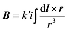
We assume the electric current is the source of the magnetic field. Parallel to our previous work [3], and geometrically speaking we then consider a looping current through a flat circle of radius R. From the symmetry of the setup one realizes that the symmetry axis of the loop, the one which is through the center and perpendicular to the loop is the only axis that the magnetic field is expressed with a one-component vector. The magnetic field of any other point off this axis would have more than one component. With this notion, in order to quantify the field we utilize a simplified version of the Biot-Savart law [4,5],
 (1)
(1)
here i is the conduction current running through the loop,  is the vector position from the current element
  to the point of interest and
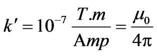 , with
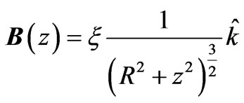
being the permeability of a vacuum. Assuming a right handed Cartesian coordinate system for a loop placed in the xy-plane with a looping counter-clock-wise current and with the z-axis being the symmetry axis through the center of the loop, Equation (1) trivially evaluates,
 (2)
(2)
where z = 2pR2ni, with n being the number of turns. For the chosen counter-clock-wise current the direction of the field remains the same on both sides of the loop; it stays oriented along the +z-axis. This is not the case for a uniform charged ring. In other words, the directions of the electric and magnetic fields are the same on one side of the loop and are opposite on the other side. Consequently, one needs to consider the corresponding electric and magnetic forces. Asides from the scaling factors for a loop of size 10.0 cm in Figure 1 we display these fields.
Figure 1 shows the magnetic field along the symmetry axis maintains its direction about the center of the loop, while the electric field changes its orientation. The electric field is asymmetrical while the magnetic field is even and symmetrical. The strengths of the fields are scaled and their units are suppressed.
Placing a negative point-like charge along the +z-axis will experience an attractive force towards the center. When it slides to the other side of the loop, according to Figure 1, it will slow down coming to a momentary stop. For a frictionless axis the energy is conserved and the process repeats itself resulting in steady oscillations. The value of the electric force causing such oscillations trivially calculates,  where q is the charge of the loose particle and the field is
 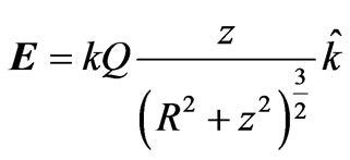 with Q being the charge on the ring; details are discussed in [3]. For a mobile permanent magnet with magnetic dipole moment
  the force can be evaluated according to
 , where the magneto static energy of the dipole in the external field is
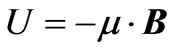 , where
  is subject to Equation (2). Placing a permanent magnet with its moment parallel and aligned with the
  field along the z-axis will experience an attractive force towards the center of the loop. The loose magnet will accelerate towards the center sliding to the other side. The magnetic field on the opposite side of the loop as shown in Figure 1 remains along the +z-axis, and it will exert a retarding force bringing the dipole to a momentary halt. Applying the gradient on the magneto static energy results in magnetic force; in other words, the inhomogeneity of the field along the z-axis is the cause of the force. Mathematically speaking, since the filed is a function of z, this yields
 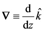 and therefore,
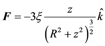
For a comprehensive understanding we plot the electric and magnetic forces. Forces are scaled and the vertical
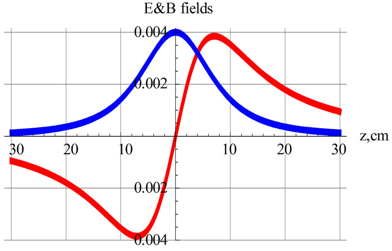
Figure 1. Display of the scaled electric field (red curve) and magnetic field (blue curve) of a uniform charged ring and a looping current of radius 10.0 cm.
axis is proportional to newtons.
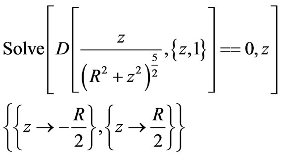
Along the positive z-axis the electric and magnetic forces both are negative; i.e. they act on the mobile pieces (either a point-like charge or a permanent magnet) attractively, pulling them towards the center of the loop. On the contrary, on the other side of the loop, i.e., along the negative z-axis, forces are positive, meaning they act towards the center causing retardation. Figure 2 also shows the electric and magnetic forces aside from their relative strengths have somewhat similar characteristics. However, the electric force has a longer effective range, while the magnetic force is relatively sharper. By inspection one learns both the electric and magnetic forces at certain specific distances from the center of the respective loops are at their extreme. For magnetic field this is,
It is also noteworthy to mention the functional form of the magnetic and the electric forces are distinctly different. For distances further from the center of the loop the magnetic field behaves as 1/distance4 while the electric field falls off as 1/distance2. Moreover, as shown in Figure 2, both forces are asymmetric about the origin; their Taylor expansions are polynomials of odd integers. Taylor expansions for electric and the magnetic forces beyond the third power (the Duffing term) are, respectively,
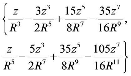
This shows the expanded functions fall off either as 1/distance2 and/or 1/distance4, respectively. To further
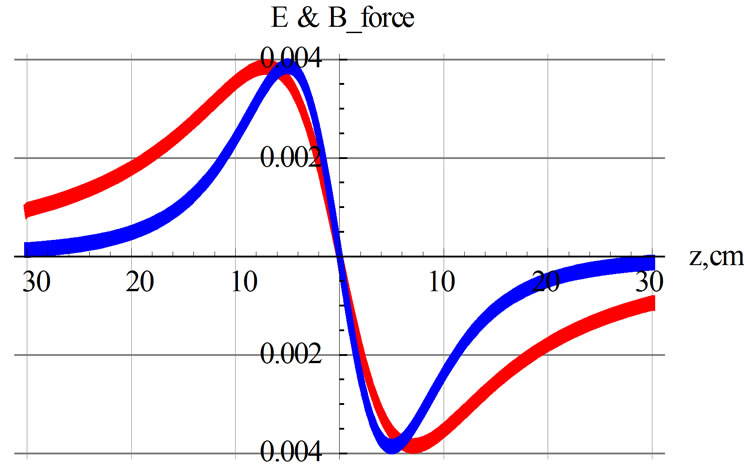
Figure 2. The red and the blue curves are the electric and magnetic forces, respectively.
our analysis we utilize the unexpanded format of the magnetic force. Its current format according to Equation (3) is a polynomial ; it contains odd powers of distance. Comparing this super structure force vs. the Duffing oscillator force that comes about from an additive perturbative z3 term to the Simple Harmonic Oscillator, i.e., az+bz3, with {a, b} being constants, one realizes the unexpanded magnetic force stretches the issues of the Duffing oscillator beyond its classic limits.
With this insight about the magnetic force we envision placing a light permanent cylindrical magnet along the horizontal symmetry axis through the center of a circular looping current. Applying Newton’s law of motion  we study its motion. This equation along the horizontal z-axis yields,
 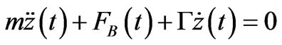 where FB and
  are the magnetic and the viscous forces, respectively. For a practical setting we envision positioning a horizontal glass tube through the center of the loop and placing the magnet in it. The air is pumped through fine in-punctured holes from underneath the tube, levitating the magnet. While the magnet under the influence of the electromagnet force slides horizontally in the tube it rubs itself against the air experiencing the viscous force. From our previous work [6] we have experience with a suitable range of variations of the viscosity coefficient G; we supply its value for our analysis.
To further the analysis of the case at hand the specification of the components in the SI units are tabulated in the values list. The R is the radius of the loop, n is the number of the turns, m is the mass of the magnet, m is its dipole moment, g = G/m is the viscosity per mass, and g is the gravity acceleration.
Figure 3 is a display the magnetic field along the symmetry axis of the looping current vs. the distance from the center of the loop.
Utilizing the magnetic force associated with this field the equation of motion yields
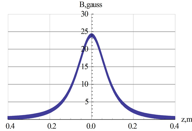
Figure 3. Display of the magnetic field along the z-axis of the looping current vs. distance from the center of the loop.
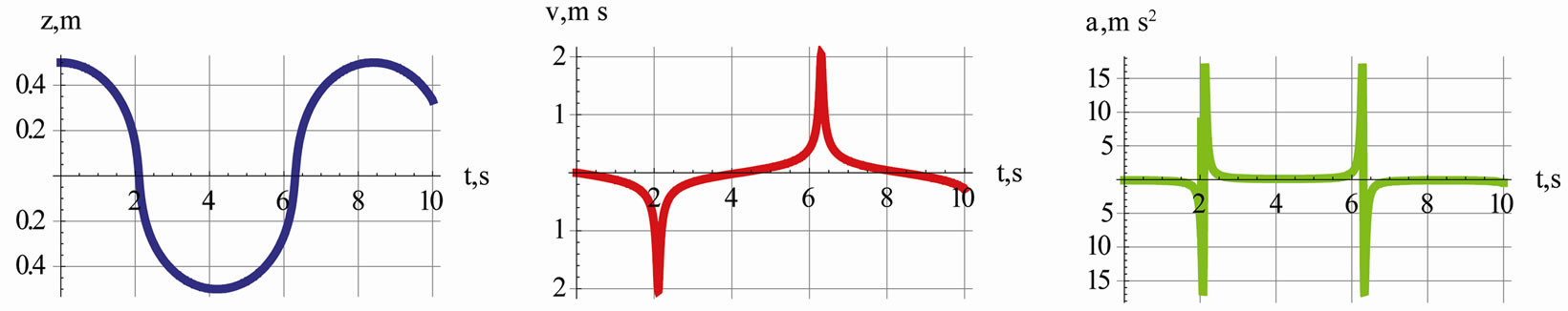
Figure 4. From left to right; display of position, velocity and acceleration of the oscillating magnetic vs. time, respectively.
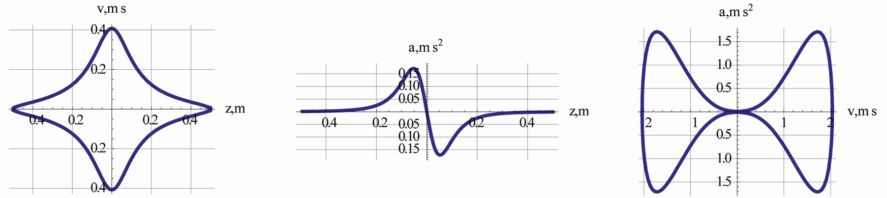
Figure 5. From left to right, the plots are associated with ,
, and
and ,respectively.
where . This is a highly nonlinear differential equation. We were unable to solve this equation analytically, so did Mathematica. We then deploy Mathematica numeric skim. Assuming a set of practical initial conditions utilizing NDSolve successfully we solve the equation. First we analyze the viscous free case.
values = {k–>1.0 × 10⁻⁷, R ® 10.5 × 10⁻², n ® 200.0, I ® 2.0, m ® 2.0 10–3, m ® 1.75, g ® 0, g ® 9.8};
Utilizing the numeric solution of the equation at hand, we form the velocity and the acceleration of the magnet. Plots of these quantities are shown in Figure 4.
The left graph of Figure 4 shows the floating magnet indeed oscillates along the symmetry axis of the looping current. A trained eye would recognize the distinct differences between the characters of these oscillations vs. the oscillations of a Simple Harmonic Oscillations (SHM). As discussed in the text, loosely speaking the magnetic force of the former is proportional to 1/z4 while the latter is proportional to z. Consequently the sinusoidal oscillations of a SHM is being replaced with a smoother “sinusoidal” function. Since, velocity and the acceleration respectively are the slopes of the position and the velocity with respect to time, the interpretation of the middle and the last plots of Figure 4 are straight forward. For instance the spikes shown in the middle graph are the extreme speeds of the oscillating magnet at the center of the loop.
Taking advantage of graphic capabilities of Mathematica by folding the time axis we display a set of phase diagrams. These are shown in Figure 5. In addition to the standard diagram, namely the plot of  we display two more “phase-type” graphs, namely plots of
 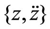 and
and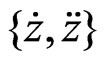 .
.
Putting all this information into perspective we close this section by mentioning that we have an understanding about how a linear oscillator oscillates; e.g. oscillations of a small angled swing, but what about oscillations of a nonlinear oscillator? To make the formulation meaningful, utilizing Mathematica animation we animate the oscillations. A snap shot of the oscillations is shown in Figure 6.
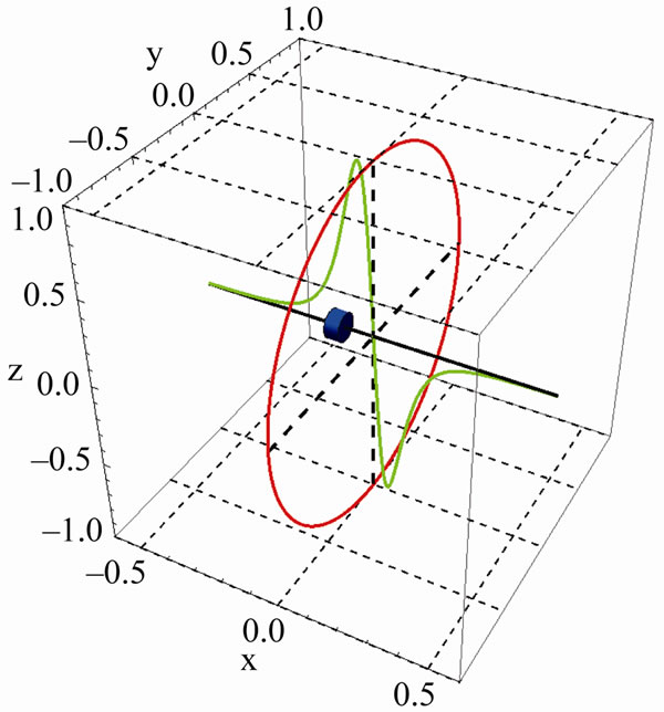
Figure 6. A snap shot of the nonlinear oscillations of the magnet (the blue cylinder). The looping current is in red and the profile of the magnetic force is the green curve.
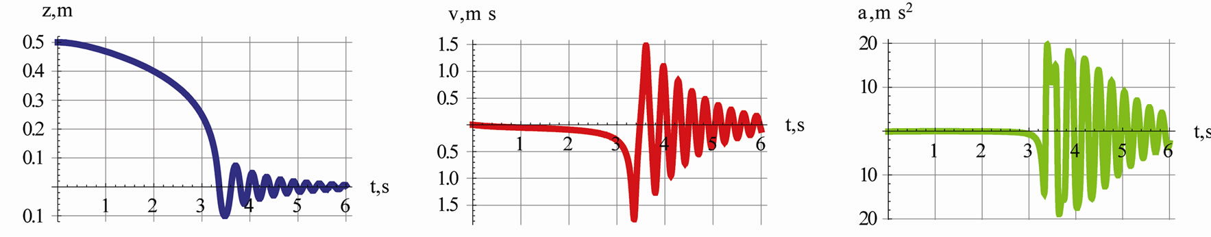
Figure 7. Description of these plots are the same as shown in Figure 4. The plots are associated with the viscous fluid with viscosity factor g = 2.0.
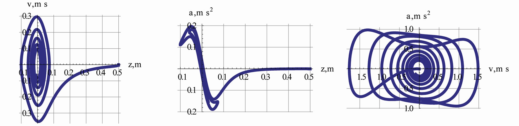
Figure 8. Description of these plots are the same as Figure 5. The plots are associated with the viscous fluid with viscosity factor g = 2.0.
4. Damped Nonlinear Oscillations
In this subsection we consider a case where in addition to the magnetic force the loose magnet along with the same previous initial conditions experiences also a speed dependent viscous force. From our previous work we utilize the value of g = G/m. Applying NDSolve we solve the associated ODE describing the motion of the magnet. Utilizing this solution we also form its associated velocity and acceleration. These are displayed in Figure 7.
Values g = {k–>1.0 × 10⁻⁷, R®10.5 × 10⁻², n ® 200.0, I ® 2.0, m ®2.0 × 10⁻³, m ® 1.75, g ® 2.0, g ® 9.8};
The impact of the viscous force is severe as expected. The viscous force dampens the oscillations bringing the oscillator to its final expected position, the center of the loop. Similar to what we discussed in the previous case, interpretation of the middle and the last graphs are straight forward.
We also plot useful graphs similar to those displayed in Figure 5. Intriguing plots such the ones shown in Figure 8 bring a greater appreciation to the power of Mathematica!
5. Exotic Designs, a Three-Ring Configuration
In this subsection we show the analysis of nonlinear oscillations may be extended to more sophisticated and interesting cases. We discuss one such case in detail and leave the design of other cases to the interest of the reader. Here we consider a set of three parallel loops separated from one another with different distances. In general the loops may have different sizes, different number of turns, different currents and they may run in different directions. For a set of parameters tabulated in the values3 list a plot of the magnetic field vs. the distance from the center of the middle loop is shown in Figure 9. A 3D plot of the setup is shown in Figure 10.
Values 3 = {k ® 1.0 × 10⁻⁷, R3 ® 20.0 × 10⁻², R1 ® 15.0 × 10⁻², R2 ® 10.0 × 10⁻², x3 ® 20.0 × 10⁻², x2 ® 10.0 × 10⁻², i3 ® 20.0, i1 ® 10.0, i2 ® 20.0, n1 ® 200.0, n2 ® 200.0, n3 ® 200.0, m ® 2.0 × 10⁻³, m ® 1.75, g ® 0.}.
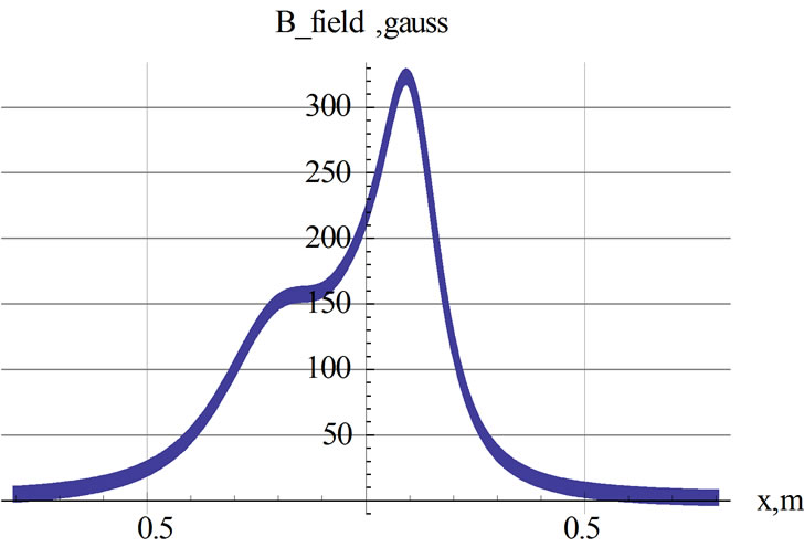
Figure 9. Plot of the magnetic field along the symmetry axis vs. the distance from the center of the middle loop. All three currents are in the same direction; two out of three currents are the same.
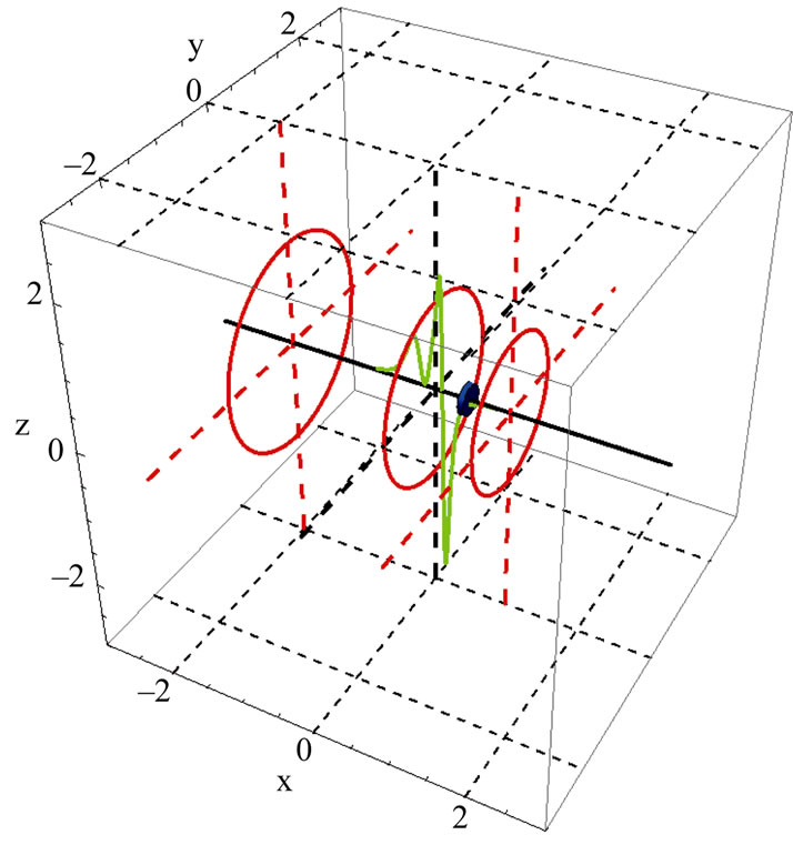
Figure 10. A 3D display of the set up. The rings are in red and the blue disk is the snap shot position of the magnet. The green curve is the profile of the distorted force.
The field along the symmetry axis is distorted. The impact of the distortion on the movement of the magnet is beyond ones intuition. To form an opinion about the movement of the magnet one needs to solve the equation of motion. We report our viscous free case and to keep the length of the manuscript manageable we do not report the cases for the viscous fluid.
As we discussed in the previous cases, with the numeric solution of the position as a function of time we form its velocity and acceleration. These quantities are shown in Figure 11.
At a first glance the time dependent position of the loose magnet, the left plot of the Figure 11 appears to be the same as its counterpart in Figure 4. However, the second and the third plots contain subtle and fine differences. The distorted spikes resemble EKG-type signals. Figure 12 is a display of a set of “phase-type” diagrams. These are quite different from their counterparts in Figure 5. The strange shape of the curves are the impact of the distorted field.
Figure 10 is a 3D plot of the setup. This plot helps to form a visual understanding about the setting. With much effort the author crafted a Mathematica code bringing the motion of the loose magnet to life. The interested readerfamiliar with Mathematica programming is encouraged crafting a code animating the motion.
6. Energy Issues
Here we consider the energy of the nonlinear oscillator. For a chosen scenario such as case 2 i.e. a single loop current and viscous fluid, the evaluation of the energy of the system is somewhat straight forward. Similarly, the energy of the different scenarios discussed in this text may also be evaluated. The energy of the mobile magnet is composed of two pieces: kinetic and potential. The total
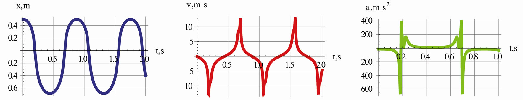
Figure 11. Description of these plots are the same as Figure 4. The differences result from the distorted magnetic field subject to Figure 9.
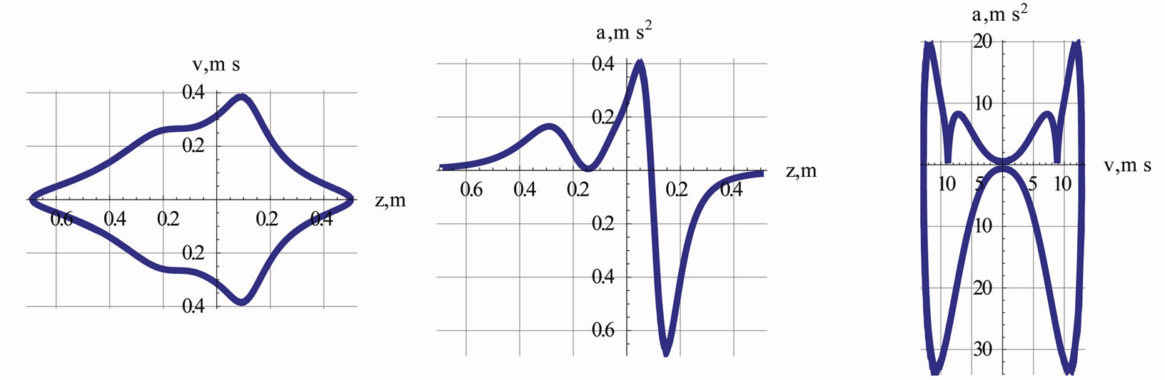
Figure 12. Description of these plots are the same as Figure 5. These plots are associated with the distorted field shown in Figure 9.
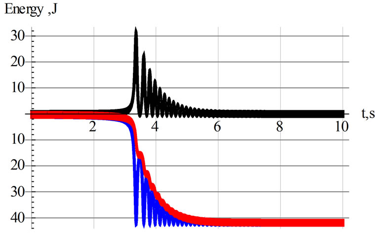
Figure 13. Plots of K.E. (the black curve) and the P.E. (the blue curve) and the total energy E (the red curve) vs. time. These are plots of viscous fluid with viscosity coefficient.γ = 2.0.
energy is E = K.E. + P.E., where 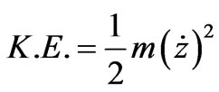 and
and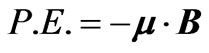 ; utilizing z(t) we evaluate
  and 1/(R^2+z^2(t))3/2 . For the case at hand the time series of the energies are shown in Figure 13.
Descriptively speaking, at the beginning the stationary magnet is far from the ring possessing a zero total energy. Under the influence of a weak magnetic field it begins being pulled towards the center of the loop. While in motion it gains kinetic and potential energies. The viscosity of the fluid dissipates the energy, dampening it to final rest position. The gradual deterioration of the energy is noticed with the jagged edges of the red curve.
7. Conclusions
Utilizing a static magnetic field we propose a design producing oscillations for a magneto static spring-mass system. A magneto-spring is made of magnetic field and inherently is a mass-less spring. This augments the classic mechanical view of the spring-mass system by passing the needed assumptions about the mass-less spring. The price we pay for our invention is the mathematical challenges we encounter with solving the nonlinear ODEs describing the motion. This by itself is a positive adventure. In light of the fast growing Computer Algebra System industry, such as Mathematica the author believes the numeric solutions are as powerful and informative as analytic ones. Had it not been for the former the insights that we gained by addressing the numeric mathematical challenges of the project at hand we would have left the problem unanswered.
The author would like to mention the current research project is a complementary analysis to our previously published work [3]. This intertwining of the parallel papers completes the analysis of truly massless-electric and magnetic spring-mass nonlinear oscillations. A thorough literature search has been completed by the author; since this project is a novel concept without previous studies, he is unable to augment the reference list beyond its current status.
8. Acknowledgements
The author would like to thank Mrs. Nenette Sarafian Hickey for carefully reading over the manuscript and making useful editorial comments.
REFERENCES
- G. Duffing, “Erzwungene Schwingungen bei Veranderlicher Eigen-frequenz,” F. Vieweg und Sohn, Braunschweig, 1918.
- S. Wolfram, “The Mathematica Book,” 5th Edition, Cambridge University Publications, Cambridge, 2003, and MathematicaTM software V8.0, 2011.
- H. Sarafian, “Static Electric-Spring and Nonlinear Oscillations,” Journal of Electromagnetic Analysis & Applications (JEMAA), Vol. 2, No. 2, February 2010, pp. 75-81.
- J. R. Retiz and F.J. Milford, “Foundations of Electromagnetic Theory,” Addison-Wesley, Hoboken, 1960.
- J. D. Jackson, “Classical Electrodynamics,” 3rd Edition, Wiley, Hoboken, 2005.
- H. Sarafian, “Dynamic Dipole-Dipole Magnetic Interaction and Damped Nonlinear Oscillations,” Journal of Electromagnetic Analysis & Applications (JEMAA), Vol. 1, No. 4, 2009, pp. 195-204.